

Technical Analysis · Lesson 08 of 15 · Reviewed November 10, 2026
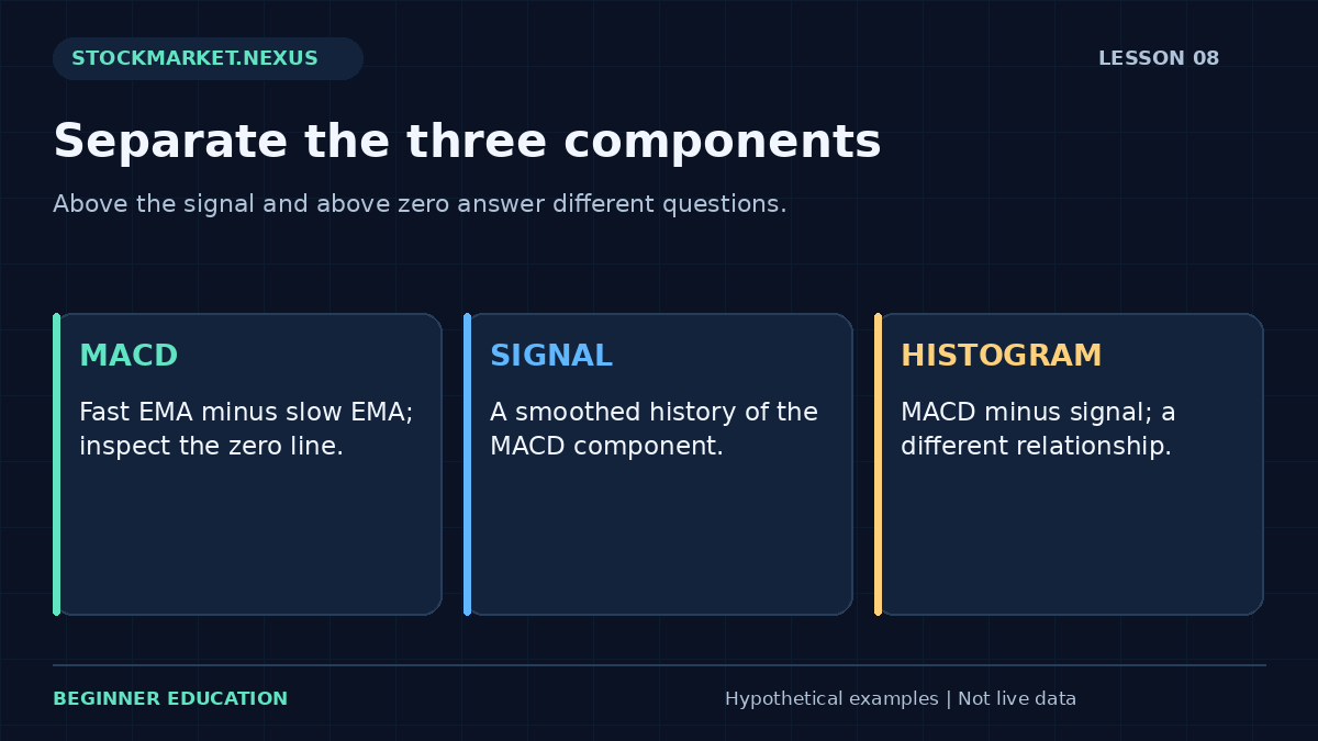
MACD stands for Moving Average Convergence Divergence. Its familiar chart panel usually contains a MACD line, a signal line, and a histogram. The components are related but answer different questions. A MACD value above zero is not the same observation as a MACD value above its signal line, and a shrinking positive histogram is not automatically a negative MACD.
This lesson separates those relationships and makes one update fully transparent. The dedicated exercise uses supplied fast and slow EMA values plus a prior signal value. It teaches the component arithmetic without pretending that a single update reconstructs a complete historical indicator or predicts the next price movement.
1. Understand the price averages behind the indicator
A common MACD configuration subtracts a 26-period EMA from a 12-period EMA and uses a 9-period EMA of the resulting MACD series as the signal line. These are familiar defaults, not universal optimal settings. The period unit follows the chart interval, so daily and intraday configurations summarize different horizons.
The MACD line is fast EMA minus slow EMA. If the fast EMA is $52 and the slow EMA is $50, MACD is +$2 in price units. If the fast EMA is $48 while the slow remains $50, MACD is −$2. The sign describes the ordering of the two selected averages.
Because both averages derive from past prices, MACD is a transformed price summary rather than a separate data source. The moving average lesson explains recursive updates, initialization, and why different historical seeds can produce early discrepancies.
2. Calculate the signal-line update
The signal line smooths MACD values. Using the common EMA multiplier convention, alpha equals 2 divided by signal period plus one. For a nine-period signal, alpha is 0.2. The updated signal equals alpha times current MACD plus one minus alpha times the prior signal.
With current MACD 2 and prior signal 1.5, the new signal is 0.2 × 2 + 0.8 × 1.5 = 1.6. This calculation requires a prior state. It does not explain how that prior signal was originally seeded or verify that the supplied fast and slow EMAs came from consistent observations.
The exercise labels these inputs explicitly. It does not take a short close list and claim to match an arbitrary chart platform’s full 12/26/9 history. A transparent component worksheet is more useful than a hidden approximation that appears precise but uses a different initialization.

3. Calculate and interpret the histogram
The histogram equals MACD minus signal. In the example, 2 − 1.6 = +0.4. A positive histogram means MACD is above its signal line. A negative histogram means MACD is below it. The histogram is a difference between two indicator components, not the stock’s trading volume.
A histogram can remain positive while shrinking. That means the gap between MACD and signal is narrowing under the selected calculation. It does not necessarily mean price is falling or MACD is below zero. Several relationships can coexist, and reading each component separately prevents contradictory descriptions.
Likewise, a negative MACD can have a positive histogram. If MACD is −1 and signal is −1.5, their difference is +0.5. The fast EMA is still below the slow EMA, while MACD is above its own smoother. These statements answer different questions and should not be compressed into a single vague label such as bullish.
4. Distinguish the two common crossings
A zero-line crossing occurs when MACD changes sign, corresponding to the fast and slow EMA ordering changing. A signal-line crossing occurs when MACD moves from one side of its signal to the other. The two events need not happen together and can have different timing.
An unfinished bar can produce a temporary crossing that disappears before completion. A rule using completed bars must wait for the selected interval to finish. A real-time rule is a different design and requires its own data and execution assumptions. A historical chart showing only final values can conceal those intrabar changes.
A crossing alone does not establish an order type, fill, holding period, or loss allowance. A professional study specifies those details separately and tests the complete method. Turning a display event into an automatic trade instruction without those definitions skips the most important operational questions.
5. Recognize scale and comparability limits
Ordinary MACD is expressed in the price units of its underlying series. A MACD value of 2 on a $20 stock is not directly comparable with 2 on a $400 stock as a standardized percentage momentum measure. The same dollar difference has a different relative scale.
Comparing MACD across instruments therefore requires care. A percentage-based oscillator would be a different calculation. Do not silently interpret ordinary MACD as though it were normalized. When comparing charts, record the security, interval, source price, periods, and axis convention.
Changes in volatility also affect the amplitude of price-derived differences. A visually dramatic histogram may reflect a larger recent price range rather than a universally stronger forecast. The ATR lesson provides a separate movement-magnitude measurement, while emphasizing that volatility does not forecast direction.
6. Understand whipsaws and overlapping evidence
In a sideways series, fast and slow averages can repeatedly change their relationship. MACD can cross its signal frequently, producing a visually busy panel. A rule that trades every crossing may accumulate spread, fees, and slippage even when price ends near its starting point.
Adding RSI or another momentum indicator does not automatically solve the problem. Several indicators may react to the same underlying changes. The added condition needs a defined purpose and a comparison showing whether it contributes useful information under realistic assumptions.
Divergence analysis has similar selection issues. Choosing the two most persuasive price and MACD peaks after seeing the future can make the pattern appear clearer than it was in real time. Define the peak-selection rule and confirmation delay before evaluating subsequent behavior.
7. Work through the MACD component exercise
Open the Lesson 8 MACD exercise. Enter fast EMA 52, slow EMA 50, previous signal 1.5, and signal period 9. Predict MACD 2, updated signal 1.6, and histogram 0.4 before calculating. The visual result should show all three component values with a visible zero reference.
Change the fast EMA to 49 while leaving the slow EMA at 50. Current MACD becomes −1. The prior signal still carries history, so the updated signal is 1.0 and the histogram is −2.0. This large negative histogram is an arithmetic consequence of the supplied transition, not a measured live-market event.
Next enter fast EMA 49, slow EMA 50, prior signal −1.5, and period 9. Updated signal becomes −1.4 and histogram +0.4. Explain why a positive histogram coexists with negative MACD. This is the central distinction the exercise is designed to teach.
8. Verify the supplied-state assumptions
The fast and slow EMA inputs should refer to the same instrument, interval end, source field, and adjustment convention. Mixing today’s fast EMA with yesterday’s slow EMA creates a number that is mathematically valid but analytically inconsistent. A calculator cannot detect every such mismatch.
The prior signal must be the preceding state under the same signal-period convention. If the period changes from nine to five, simply keeping an old nine-period prior state creates a teaching scenario rather than a correctly reconstructed five-period history. The tool allows parameter experiments but describes them as supplied-state updates.
For platform reconciliation, use enough earlier observations and document initialization. Check rounding only after checking the underlying definitions. A small displayed difference can result from hidden decimal precision, while a large difference often points to mismatched settings or histories.
9. Write a testable MACD research question
A useful statement might examine a completed signal-line crossing under a specified wider structure and measure the next five-session return under a defined execution assumption. It should identify whether the zero-line state is a filter, how repeated crossings are handled, and when a position exits.
Keep the comparison simple enough to understand. If dozens of filters are added until a backtest looks attractive, the final rule can fit historical noise. Preserve every tested version and reserve unseen observations for later evaluation. The course’s backtesting lesson explains why the selection process itself is part of the evidence.
Include unfavorable cases, transaction costs, and periods with no position. A strategy that looks successful during one sustained trend may behave very differently in a range. Reporting exposure, turnover, drawdown, and the baseline gives a more complete picture than a collection of successful crossings.
10. Use the panel as a readable calculation
You should be able to calculate all three components, explain the zero line, distinguish signal crossings from zero crossings, and identify why a negative MACD can have a positive histogram. You should also recognize that a supplied-state worksheet is not a full historical reconstruction.
A professional MACD note states the specific relationships and settings before proposing an interpretation. This makes the analysis easier to audit and avoids treating a familiar visual panel as an independent authority. The arithmetic is useful precisely because its scope and limitations remain visible.
Case review: positive histogram below zero
Take fast EMA 49, slow EMA 50, previous signal −1.5, and signal period nine. MACD is −1. The updated signal is −1.4 and histogram is +0.4. The fast EMA remains below the slow EMA, while MACD is above its smoother. Both statements belong in the description.
Calling the entire panel positive would hide the negative MACD; calling it entirely negative would hide the positive histogram. The most accurate note states each relationship and avoids compressing several measurements into one emotional label. A component chart with a zero reference makes the distinction visible.
Next increase only the fast EMA to 50. MACD becomes zero, the supplied-state signal becomes −1.2, and the histogram becomes +1.2. That is a controlled arithmetic experiment, not a reconstructed market sequence, because the prior signal was held fixed deliberately. Explain that limitation in the review. Parameter experiments are useful when their artificial assumptions remain explicit rather than being presented as historical evidence.
A repeatable practice and review protocol
Before changing the example, write down the question you expect the calculation to answer. Copy the input values, units, chronological order where relevant, and the observation time. State whether the values are fictional, historical, or current. The exercises in this course begin with fictional data so the arithmetic can be studied without implying that a real security offers a particular opportunity. A calculator result is only as meaningful as its input definitions.
Predict the direction of one change before pressing the calculation button. Change one input at a time, explain which part of the formula it affects, and compare the result with your prediction. This controlled approach is more informative than changing several fields until an attractive number appears. If the result surprises you, return to the definition and denominator before looking for a market explanation. Arithmetic mistakes and interpretation mistakes require different corrections.
Then test an ordinary alternative and an edge case. An ordinary alternative checks whether you understand the relationship away from the default example. An edge case checks whether a ratio becomes undefined, a sample becomes insufficient, or an input ordering becomes impossible. A clear validation message is a useful result. Do not work around it by entering an unrelated value merely to make the screen produce an answer. First understand which assumption the rejected value violated.
Save a short review with four parts: the observation, the calculation, the interpretation, and the unresolved limitation. Keep those parts separate. The observation records what the supplied data says; the calculation shows how the number was obtained; the interpretation is a conditional hypothesis; the limitation identifies information the exercise does not provide. This structure makes the note understandable to another beginner and makes later revisions easier to audit.
If you extend the example into a paper-trading study, define signal time, decision time, order assumptions, quantity, costs, and review horizon before checking the outcome. Preserve the original version. Record unfavorable cases and skipped cases under the same rules as favorable ones. A chart image can support the record, but it should not replace the actual values and definitions. A successful-looking historical picture is not a substitute for a complete sample.
Finish by explaining the result in plain language without using a pattern name as the explanation. Identify what changed, what stayed fixed, and what the exercise still cannot establish. You have completed the practice when you can reproduce the important arithmetic, recognize an invalid comparison, and describe an alternative outcome. Repeating this process across the course builds a consistent analytical habit while keeping the different formulas and their limitations distinct.
Sources and calculation notes
Primary educational background provides additional context for the topic. The fictional examples, teaching cases, diagrams, and worksheets here are original educational illustrations. Calculation conventions and missing information are stated explicitly; indicator readings do not establish future returns.