

Technical Analysis · Lesson 15 of 15 · Reviewed November 10, 2026
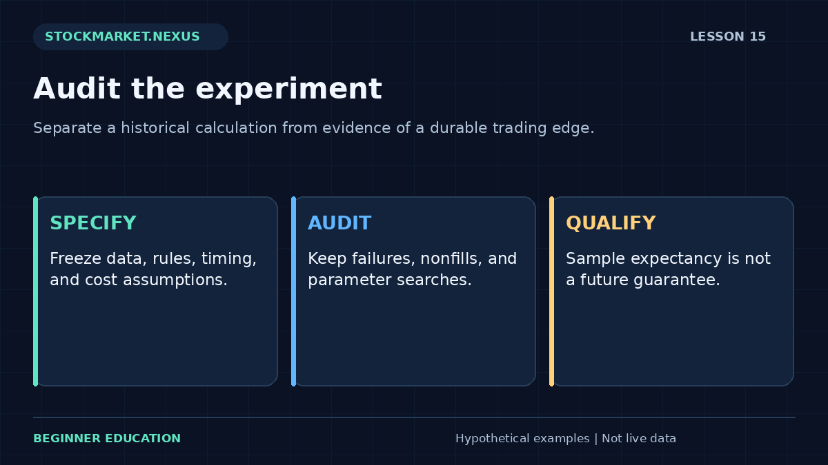
A backtest applies defined rules to historical information under stated assumptions. It can help expose arithmetic errors, operational ambiguities, and weaknesses in a hypothesis. It cannot turn a selected historical result into a guarantee of future profit. The quality of the experiment depends on the data, timing, selection process, execution model, and honesty of the review.
This lesson introduces a practical audit framework and a dedicated sample-economics worksheet. The tool calculates gross and net results, average net outcome, win rate, and a simplified break-even win rate from hypothetical summary inputs. It is an arithmetic exercise, not a complete backtesting engine or a statistical certification of an edge.
1. Write the complete rule before collecting examples
Define the eligible instruments, dates, timeframe, session, source prices, indicator settings, signal conditions, entry timing, exit rule, and cost model. Include what happens when data is missing, an order does not fill, or both a target and stop lie inside one bar. A strategy described only by a pattern name is not ready for a reproducible test.
The rule should identify information availability. A signal requiring a completed close cannot justify an earlier fill inside that same bar. A pivot requiring later confirmation cannot be treated as known at the turning point. These timing errors can make a historical method appear more accurate than it could have been in practice.
Start with the small, explicit questions developed in technical analysis for beginners. A narrow rule is easier to audit than a large collection of discretionary judgments assembled after seeing outcomes.
2. Define the eligible population and preserve failures
A collection of memorable winning charts is not a backtest because it lacks the denominator of all eligible cases. Begin with a predefined population and apply the same rule across it. Keep failed signals, ordinary cases, nonfills, and instruments that later disappeared from the current market universe.
Survivorship bias occurs when historical analysis includes only instruments that survived or remain available today. Delisted or failed securities may have been part of the original opportunity set. Excluding them can materially alter results. Data limitations should be documented rather than disguised as a cleaner universe.
Selection bias also appears when examples are chosen because their eventual outcomes are known. If a researcher reviews a large chart archive and keeps only textbook patterns, the final sample may say more about the selection process than the rule. Record how every observation entered the study.
3. Model execution with appropriate humility
Historical reference prices are not automatically available fills. A market order can cross a spread and experience slippage. A limit order can remain unfilled or fill partially. An opening gap can bypass a planned protective price. A credible study states the instruction and uses assumptions that the available data can support.
Bar data creates sequence ambiguity. If one bar reaches both a stop and target, OHLC alone may not show which came first. Finer data can help, but it also has coverage and quality limits. A conservative convention or an unresolved-case label is more honest than always assuming the favorable path.
Review bid-ask spreads and slippage before interpreting small average gains. A strategy with frequent trades can lose its apparent advantage after modest friction. Costs should be included before presenting net results, not added as an afterthought.
4. Separate gross trade outcomes from charges
The worksheet asks for the number of gross winning trades, number of gross losing trades, average gross win, average gross loss magnitude, and fixed cost per completed trade. It assumes no breakeven trades in this simplified sample. Every trade pays the entered cost, including gross winners and gross losers.
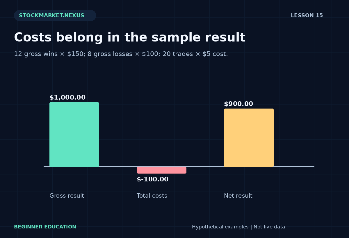
Suppose there are 12 gross winners averaging $150 and eight gross losers averaging $100, with $5 cost per trade. Gross gains total $1,800 and gross losses total $800, leaving gross result $1,000. Twenty completed trades incur $100 total cost, so net result is $900.
The sample average net outcome is $900 divided by 20, or $45 per trade. This is a historical sample statistic under the supplied inputs. It is not a forecast that the next trade will earn $45, and it contains no estimate of uncertainty, path, or capital requirements.
5. Calculate win rate and break-even win rate
Gross win rate is gross winners divided by total trades. In the example, 12/20 is 60%. The simplified net break-even win rate solves p times average win minus one minus p times average loss minus per-trade cost equals zero. It is (average loss plus cost) divided by average win plus average loss.
With average win $150, average loss $100, and cost $5, the break-even fraction is 105/250, or 42%. This threshold assumes those average outcomes and costs remain fixed. A changing distribution, variable costs, breakeven trades, or position-size differences would require a more detailed model.
A high win rate alone does not establish attractive economics. Frequent small gains can be outweighed by rare large losses. Conversely, a lower win rate can have positive sample economics when average wins exceed losses sufficiently. Report outcome sizes and costs alongside the rate rather than using win rate as a standalone quality score.
6. Understand what summary statistics omit
The same count and average outcomes can arise from very different sequences. Ten losses in a row and alternating wins and losses can produce the same final total while creating different drawdowns and practical pressures. The summary worksheet does not calculate a path-based maximum drawdown because it does not receive ordered individual trade results.
It also does not know exposure, holding periods, overlapping positions, cash constraints, taxes, financing, or capital changes. A sample total of $900 cannot be converted into a meaningful account return without a denominator and cash-flow convention. Precision in one statistic does not fill in missing information elsewhere.
A full review should retain individual observations and timestamps. Summary calculations are useful checks, but the underlying ledger is needed to investigate anomalies, sequence risk, and changing conditions. Keep raw records rather than only the final dashboard.
7. Use the dedicated sample-audit exercise
Open the Lesson 15 backtesting exercise. Enter 12 gross winners, eight gross losers, average gross win 150, average gross loss 100, and cost per trade 5. Predict gross result 1000, total cost 100, net result 900, average net outcome 45, gross win rate 60%, and break-even rate 42%.
Increase cost to 60. Total cost becomes 1200 and net result becomes negative 200, despite the unchanged 60% gross win rate. The break-even rate rises to 64%. This isolates the effect of costs without changing the selected historical outcomes.
Try a sample with zero trades; the calculator should reject an undefined average. Counts must be nonnegative whole numbers, and average win and loss magnitudes must be positive. If the entered cost exceeds the average gross win, the simplified break-even rate can exceed 100%, revealing that the supplied fixed economics cannot break even through win frequency alone.
8. Track parameter searches and overfitting
A rule selected from hundreds of indicator combinations has had many opportunities to fit historical noise. Reporting only the best result hides that search. Keep a research log listing tested periods, thresholds, filters, and rejected versions. The selection process is part of the evidence.
Reserve genuinely unseen observations for later evaluation, and avoid repeatedly using the same holdout to revise the rule. Once it influences design choices, it is no longer untouched evidence. A forward paper study can help test operational clarity, although simulated fills still differ from actual execution.
The paper-trading guide provides a structured way to practice without treating simulated profits as proof of live performance. The objective is to expose unclear rules and inconsistent behavior before drawing strong conclusions.
9. Compare with a suitable baseline
A positive strategy result during a broad advance may reflect market exposure rather than useful timing. Compare against a relevant baseline under consistent dates, costs, and return conventions. Consider exposure, idle cash, turnover, drawdown, and concentration rather than only final profit.
A benchmark comparison also needs care. A price-only strategy series and a total-return benchmark use different conventions. Different currencies or observation times can distort the result. State those choices and avoid selecting the benchmark after seeing which one makes the strategy look best.
Break the sample into meaningful subperiods without using those subdivisions merely to discard unfavorable regimes. A method that depends entirely on one short episode deserves a narrower conclusion than one with broadly consistent behavior. Neither result guarantees that future conditions will resemble the past.
10. Write conclusions that match the experiment
A defensible conclusion might say, “Under these rules, data, and cost assumptions, this historical sample produced the following net outcomes; the study does not establish future profitability.” It should identify the largest unresolved limitations and preserve enough detail for another person to reproduce the calculation.
You should be able to calculate sample economics, explain the break-even formula, identify look-ahead and survivorship bias, and distinguish a summary worksheet from a full backtest. The professional benefit of backtesting is disciplined questioning. A disappointing result can be useful when it prevents an unsupported belief from becoming a larger commitment.
Case review: identical expectancy, different sequences
Imagine two hypothetical ledgers with the same 12 gross wins, eight gross losses, average win 150, average loss 100, and cost 5. One ledger begins with eight losses; the other alternates losses among wins. The summary worksheet produces the same net result and average outcome for both, but their drawdown paths differ.
The tool is correct to omit a maximum-drawdown claim because it does not receive the ordered ledger. Adding such a statistic from counts and averages alone would invent information. A professional dashboard should distinguish unavailable measurements from zero values: unknown drawdown is not zero drawdown.
For the review, list which additional data would be required to evaluate path risk, exposure, and account return. At minimum, preserve ordered trade outcomes, timestamps, quantities, capital assumptions, and cash flows where relevant. This case demonstrates the appropriate role of a summary exercise. It is an arithmetic audit that can reveal inconsistencies, while a complete backtest requires a richer record and a documented selection and execution process.
A repeatable practice and review protocol
Before changing the example, write down the question you expect the calculation to answer. Copy the input values, units, chronological order where relevant, and the observation time. State whether the values are fictional, historical, or current. The exercises in this course begin with fictional data so the arithmetic can be studied without implying that a real security offers a particular opportunity. A calculator result is only as meaningful as its input definitions.
Predict the direction of one change before pressing the calculation button. Change one input at a time, explain which part of the formula it affects, and compare the result with your prediction. This controlled approach is more informative than changing several fields until an attractive number appears. If the result surprises you, return to the definition and denominator before looking for a market explanation. Arithmetic mistakes and interpretation mistakes require different corrections.
Then test an ordinary alternative and an edge case. An ordinary alternative checks whether you understand the relationship away from the default example. An edge case checks whether a ratio becomes undefined, a sample becomes insufficient, or an input ordering becomes impossible. A clear validation message is a useful result. Do not work around it by entering an unrelated value merely to make the screen produce an answer. First understand which assumption the rejected value violated.
Save a short review with four parts: the observation, the calculation, the interpretation, and the unresolved limitation. Keep those parts separate. The observation records what the supplied data says; the calculation shows how the number was obtained; the interpretation is a conditional hypothesis; the limitation identifies information the exercise does not provide. This structure makes the note understandable to another beginner and makes later revisions easier to audit.
If you extend the example into a paper-trading study, define signal time, decision time, order assumptions, quantity, costs, and review horizon before checking the outcome. Preserve the original version. Record unfavorable cases and skipped cases under the same rules as favorable ones. A chart image can support the record, but it should not replace the actual values and definitions. A successful-looking historical picture is not a substitute for a complete sample.
Finish by explaining the result in plain language without using a pattern name as the explanation. Identify what changed, what stayed fixed, and what the exercise still cannot establish. You have completed the practice when you can reproduce the important arithmetic, recognize an invalid comparison, and describe an alternative outcome. Repeating this process across the course builds a consistent analytical habit while keeping the different formulas and their limitations distinct.
Sources and calculation notes
Primary educational background provides additional context for the topic. The fictional examples, teaching cases, diagrams, and worksheets here are original educational illustrations. Calculation conventions and missing information are stated explicitly; indicator readings do not establish future returns.