

Technical Analysis · Lesson 03 of 15 · Reviewed November 10, 2026
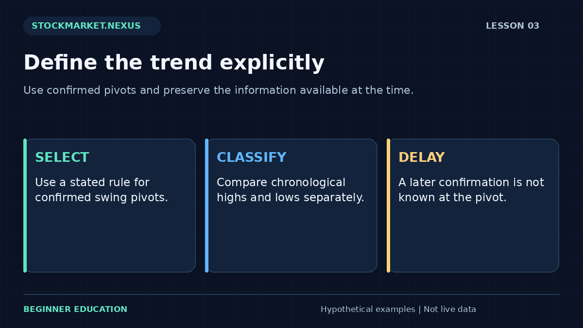
A trend description summarizes the relationship among selected price swings. An upward sequence is commonly associated with higher highs and higher lows; a downward sequence with lower highs and lower lows. Those phrases are easy to repeat, but they become useful only after you define which highs and lows count, when they are confirmed, and which timeframe they describe.
This lesson turns visual trend language into an explicit classification exercise. It does not attempt to predict the next swing. The objective is to describe a sequence consistently, identify mixed evidence, and preserve the delay between a possible turning point and the moment a chosen confirmation rule makes it knowable.
1. Distinguish individual bar extremes from swing pivots
Every ordinary bar has a high and low, but not every bar extreme is a meaningful swing pivot. A pivot-selection rule filters a sequence into selected turning points. One possible rule labels a high only after a specified number of later bars have lower highs. Another uses a defined price reversal. These methods select different points and have different delays.
A rule requiring two later bars cannot confirm today’s potential high today. The high may ultimately be plotted on today’s date, but the information needed to label it arrives later. A historical chart can hide that delay by drawing the label backward at the turning point. A backtest that trades on the pivot date without the confirmation delay uses future information.
For the dedicated exercise, the learner supplies already confirmed swing highs and already confirmed swing lows, each in chronological order. The tool classifies those supplied values. It does not discover pivots, verify their timing, or claim that a plotted turning point was tradable at its exact extreme.
2. Define an upward sequence precisely
Suppose three confirmed highs are $50, $53, and $56, while the corresponding chronological low sequence is $46, $48, and $51. Every later high exceeds the previous high, and every later low exceeds the previous low. Under the worksheet’s strict rule, that is an upward structure across the supplied observations.
The word “strict” matters. Equal highs or equal lows do not qualify as increasing in this exercise. Some discretionary methods allow tolerance zones for nearly equal pivots, but such a tolerance must be specified in price units or percentages. Otherwise one analyst may call the sequence rising while another calls it flat, with neither using the same definition.
An upward classification describes the chosen sample. It does not guarantee continued appreciation, establish a favorable entry, or measure the depth of possible drawdowns. A sequence can remain upward while the latest pullback is large enough to create a substantial loss for someone who entered near the most recent high.

3. Define a downward sequence with the same discipline
Now use highs $56, $53, and $50 and lows $51, $48, and $45. Both sequences decrease strictly. The worksheet labels downward structure. This describes declining selected reference points, not a recommendation to sell short. Short positions involve separate execution, borrowing, account, and loss considerations that the classifier does not model.
A lower high alone does not establish the complete downward pattern under this definition. A security might form a lower high while its lows continue rising, creating compression. Likewise, one new low inside an otherwise rising sequence does not automatically settle every longer-term trend question. The classifier should report the evidence it has rather than force a directional verdict.
Comparing trend descriptions requires matching the selection method and interval. A daily upward sequence can coexist with an intraday downward sequence. The descriptions refer to different scales. Resolve the apparent conflict by identifying the timeframe and decision horizon rather than declaring one chart correct and the other irrelevant.
4. Mixed structure is a useful result
Highs $50, $53, and $52 with lows $46, $48, and $49 do not meet either complete directional rule. The high sequence first rises and then falls, while the low sequence rises. “Mixed” is an informative classification because it tells the learner that the supplied evidence is not a clean monotonic sequence.
Sideways ranges, expanding formations, and transitional structures can all produce mixed results. The worksheet does not try to assign every named chart pattern. That restraint prevents a small numerical exercise from pretending to provide a comprehensive market diagnosis. A separate study could define additional categories, but each category would need clear rules.
A mixed label can support a decision to observe longer in a paper exercise. It should not trigger random changes to the pivot rule until a directional label appears. Changing definitions in response to discomfort makes the classification less reproducible and makes later performance claims harder to evaluate.
5. Add magnitude without confusing it with direction
The difference between the first and last supplied high gives one measure of high-sequence change. Percentage change divides that difference by the first high. The same calculation can be applied to the low sequence. These measures help compare scale, but they omit the path between the endpoints and should not replace the full sequence.
For highs $50 to $56, endpoint change is 12%. For lows $46 to $51, it is approximately 10.87%. Neither percentage is a realized trade return because no entry, exit, quantity, or cost has been specified. A pivot high is also not necessarily an executable purchase or sale price available after confirmation.
A very small higher high can satisfy a strict rule while being economically minor relative to spread and volatility. A large advance can create a strong upward classification while leaving a new entry far from a reasonable invalidation scenario. Direction, magnitude, execution, and risk are separate dimensions of the review.
6. Use moving averages as a different description
A moving average summarizes selected observations, while pivot structure summarizes selected turning points. They can disagree without either calculation being wrong. A recent close may fall below a short moving average while the latest confirmed swing low remains above the previous confirmed low.
If a method combines these descriptions, define their roles. One might establish the wider structure and the other provide a timing filter. Test whether the added filter improves a predefined outcome after costs rather than assuming more conditions create better evidence. The moving average lesson explains how periods and smoothing affect the displayed line.
Avoid calling two price-derived descriptions independent confirmation without examining their overlap. Both may respond to the same recent change. Agreement can make a narrative feel stronger even when it adds little distinct information. A research notebook should record what each component contributes to the actual decision rule.
7. Work through the pivot classifier
Open the Lesson 3 trend structure exercise. Enter highs 50, 53, 56 and lows 46, 48, 51, ordered oldest to newest. The result should identify both increasing sequences and show the upward classification. The chart connects supplied highs and lows separately; it does not reconstruct the full market path between them.
Change the final high to 52. The low sequence still rises, but the high sequence is no longer strictly increasing. The classification becomes mixed. Explain that change before relying on the label. Next enter three equal highs and three equal lows. The strict classifier should again avoid calling the structure upward or downward.
Finally reverse both original sequences. The classification becomes downward. Notice that reversing a list is a mathematical demonstration, not a legitimate way to analyze a live chart. Real observations must remain chronological. A tool cannot know whether the user entered the correct chronology, so the exercise states that responsibility clearly.
8. Connect trend analysis to a chart plan
Imagine a fictional daily chart with a completed higher low near $48 and a later close at $54. A learner may study whether continuation occurs, but the $6 distance to the earlier low has practical consequences. A plan that ignores that distance because the trend looks attractive has not yet translated analysis into exposure.
An invalidation level should reflect the hypothesis being studied. If the hypothesis concerns the latest confirmed structure, a move through a selected reference may weaken it. But the price at which an exit actually fills can differ from that reference, especially around gaps or thin liquidity. The lesson on technical levels and position risk models this distinction explicitly.
A trendline is another chosen representation, not an objective barrier. Its slope depends on the anchor points and chart scale. Moving an anchor after every violation can make a historical drawing look remarkably accurate while concealing that the rule changed. Preserve original drawings and distinguish revisions from the initial plan.
9. Avoid confirmation and hindsight traps
A common hindsight error is selecting the “important” swings only after seeing the full advance. Small failed structures disappear from the story while successful large swings remain. A reproducible method needs a selection rule that could operate with information available at each point in time.
Another trap is using the final revised indicator history as though it were the real-time display. Some swing-detection tools revise their most recent points as new prices arrive. If a tool can repaint a tentative pivot, record the tentative status and the later confirmation time. A polished historical line can otherwise imply a certainty that was absent live.
The same principle applies across timeframes. A weekly high or low is not final midway through the week. If a daily decision uses the current week’s evolving structure, say so. For a longer-horizon perspective on this interaction, see daily and weekly chart structure.
10. Review a classification as a description, not a forecast
A useful journal records the supplied pivots, their dates, their confirmation dates, the selection rule, the timeframe, and the resulting label. It also records mixed cases. Without those cases, a learner cannot tell whether the method classifies most observations cleanly or only a small selected subset.
After the study horizon, compare the subsequent path with the original hypothesis. A continuing rise does not validate every upward classifier, and a reversal does not invalidate the arithmetic. The question is whether a predefined rule, applied consistently across a suitable sample, adds useful information beyond an appropriate baseline.
You are ready to continue when you can explain a mixed result, identify confirmation delay, and distinguish a pivot endpoint percentage from a trade return. Those habits keep trend analysis grounded in observable structure and prevent a helpful chart description from becoming an unsupported promise about the future.
Case review: a pivot that was not yet confirmed
A fictional high occurs on Monday at $56. The selected rule requires the next two completed daily highs to remain below it. Tuesday finishes below $56, but the condition is still incomplete. Wednesday also finishes below it, so the high becomes confirmed only after Wednesday’s chosen session ends. Plotting the label on Monday does not move that information backward in time.
If a historical study assumes a sale at Monday’s high because the final chart shows a confirmed pivot there, it has used Wednesday’s information to justify Monday’s action. A more honest study records both the pivot date and confirmation date, then applies a plausible later decision rule.
Repeat the case with Wednesday making a new high instead. The Monday candidate no longer satisfies the original rule. Keep that failed candidate in the research notes if the study tracks tentative pivots. The point is not to find a confirmation method with no delay; confirmation necessarily depends on information. The point is to make the delay visible so a clean historical structure is not mistaken for real-time certainty.
A repeatable practice and review protocol
Before changing the example, write down the question you expect the calculation to answer. Copy the input values, units, chronological order where relevant, and the observation time. State whether the values are fictional, historical, or current. The exercises in this course begin with fictional data so the arithmetic can be studied without implying that a real security offers a particular opportunity. A calculator result is only as meaningful as its input definitions.
Predict the direction of one change before pressing the calculation button. Change one input at a time, explain which part of the formula it affects, and compare the result with your prediction. This controlled approach is more informative than changing several fields until an attractive number appears. If the result surprises you, return to the definition and denominator before looking for a market explanation. Arithmetic mistakes and interpretation mistakes require different corrections.
Then test an ordinary alternative and an edge case. An ordinary alternative checks whether you understand the relationship away from the default example. An edge case checks whether a ratio becomes undefined, a sample becomes insufficient, or an input ordering becomes impossible. A clear validation message is a useful result. Do not work around it by entering an unrelated value merely to make the screen produce an answer. First understand which assumption the rejected value violated.
Save a short review with four parts: the observation, the calculation, the interpretation, and the unresolved limitation. Keep those parts separate. The observation records what the supplied data says; the calculation shows how the number was obtained; the interpretation is a conditional hypothesis; the limitation identifies information the exercise does not provide. This structure makes the note understandable to another beginner and makes later revisions easier to audit.
If you extend the example into a paper-trading study, define signal time, decision time, order assumptions, quantity, costs, and review horizon before checking the outcome. Preserve the original version. Record unfavorable cases and skipped cases under the same rules as favorable ones. A chart image can support the record, but it should not replace the actual values and definitions. A successful-looking historical picture is not a substitute for a complete sample.
Finish by explaining the result in plain language without using a pattern name as the explanation. Identify what changed, what stayed fixed, and what the exercise still cannot establish. You have completed the practice when you can reproduce the important arithmetic, recognize an invalid comparison, and describe an alternative outcome. Repeating this process across the course builds a consistent analytical habit while keeping the different formulas and their limitations distinct.
Sources and calculation notes
Primary educational background provides additional context for the topic. The fictional examples, teaching cases, diagrams, and worksheets here are original educational illustrations. Calculation conventions and missing information are stated explicitly; indicator readings do not establish future returns.