

Technical Analysis · Lesson 14 of 15 · Reviewed November 10, 2026
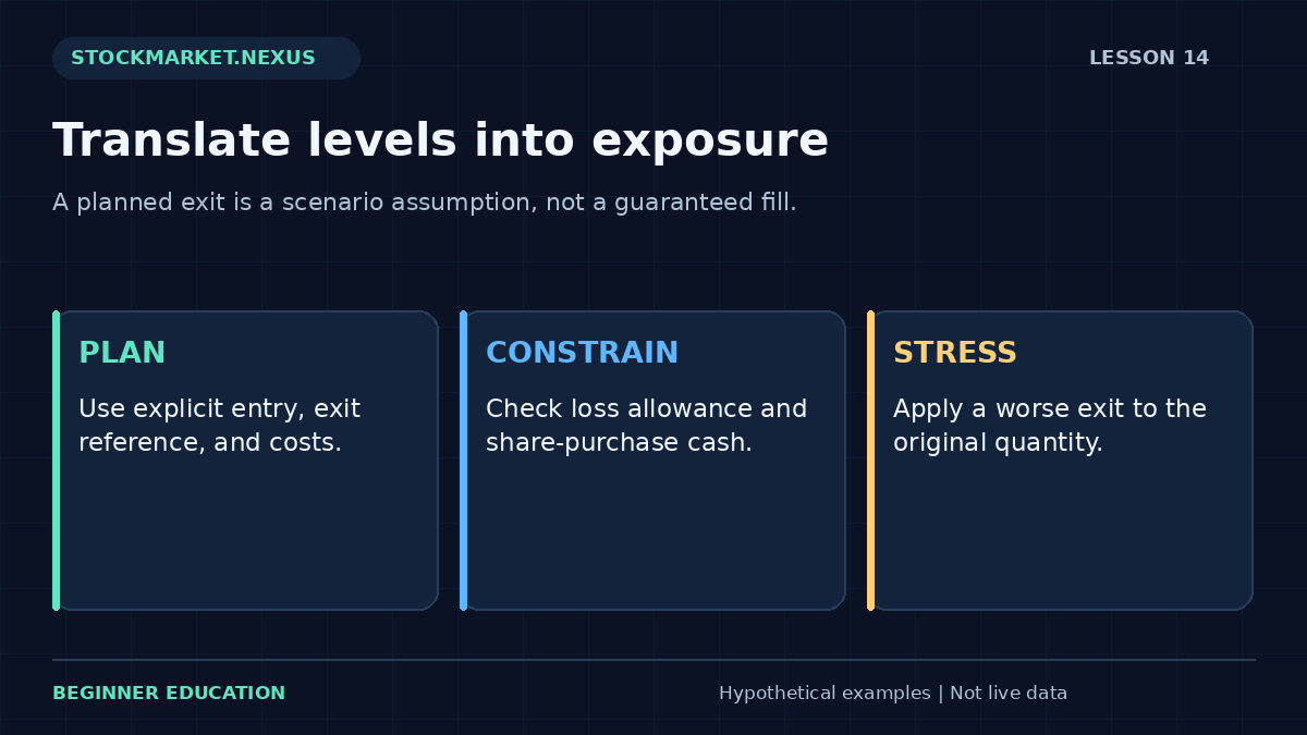
A chart level becomes operationally meaningful only when it is connected to a hypothesis, an entry assumption, an exit instruction, quantity, costs, and the possibility of worse execution. Drawing a line below price does not establish a maximum loss. A professional plan separates the intended reference from the cash exposure that different fills could create.
This lesson uses a long-share educational scenario to translate technical distances into a hypothetical whole-share quantity. It then applies a separate stressed exit to that same quantity. The worksheet is a planning demonstration, not a personalized size recommendation, and it does not model leverage, short sales, derivatives, taxes, or every brokerage restriction.
1. Define the hypothesis before choosing the loss distance
An invalidation reference should relate to the observation being studied. A hypothesis about a breakout holding above a prior range might use a different reference from a hypothesis about a longer sequence of rising swing lows. If the reference is chosen only to make a preferred quantity affordable, the chart analysis has become a justification rather than a test.
Write the hypothesis in measurable terms and identify what would weaken it. This might be a completed close inside a prior range or a price crossing a selected boundary. Those are different observation rules with different timing. A completed-close invalidation cannot guarantee an earlier intraday exit at that close’s eventual value.
The support and resistance lesson explains how to document reference areas without pretending they control the market. This lesson assumes the learner has already chosen a reference and focuses on its exposure consequences.
2. Separate entry, planned exit, and actual exit
Entry is the assumed purchase fill in the worksheet. Planned exit is the hypothetical reference used for the initial loss-distance calculation. Stressed exit is a separate adverse fill scenario. Keeping all three visible prevents a planned boundary from being mistaken for an insured execution price.
Suppose entry is $50, planned exit $48, and stressed exit $45. Planned price loss is $2 per share; stressed price loss is $5 per share. A stop order or alert near $48 does not make the $45 scenario impossible. A gap, halt, or thin market can prevent a fill at the reference.
An actual order also needs type, duration, activation convention, and quantity. A stop-market order prioritizes execution after activation under its rules, while a stop-limit can remain unfilled if the limit cannot be satisfied. Review market, limit, and stop orders before treating a chart plan as a complete execution plan.
3. State the hypothetical loss allowance and cash limit
The worksheet accepts an entered loss allowance, available cash, total fixed round-trip charges, entry, planned exit, target, and stressed exit. The allowance is a user-supplied scenario amount, not a recommendation about what any person should risk. Financial circumstances and suitability are outside the exercise.
For the initial whole-share calculation, charges are subtracted from the allowance before dividing by planned per-share loss. This leaves room for the entered fixed costs in the modeled planned loss. If the allowance does not exceed the charges, no shares fit under this convention.
A separate cash constraint limits shares to available cash divided by entry price, rounded down. In this simplified worksheet, available cash is explicitly cash reserved for the share purchase; round-trip charges are handled in the separate loss calculation. It is not a complete settlement or buying-power model, and the input instructions state that distinction.
4. Calculate the whole-share quantity transparently
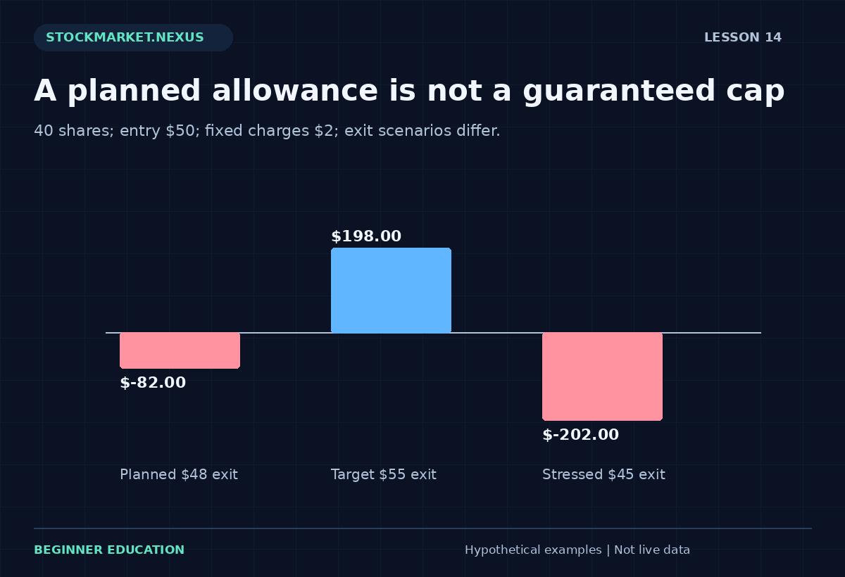
With allowance $100, fixed charges $2, entry $50, and planned exit $48, the loss-limited quantity is floor(($100 − $2) ÷ $2), or 49 shares. If share-purchase cash is $2,000, the cash-limited quantity is floor($2,000 ÷ $50), or 40 shares. The worksheet uses the smaller quantity: 40.
Planned net loss at that quantity is 40 × $2 + $2 = $82. Entry share value is $2,000. The unused allowance is not an instruction to increase exposure; it is a consequence of the cash constraint and whole-share rounding. A model should show zero when no whole share fits rather than rounding upward.
Different fee structures require different formulas. Per-share commissions, minimum charges, financing, and variable execution costs are not fully represented by one fixed total. The entered charge should be treated as a scenario assumption and reviewed for the intended educational example.
5. Calculate planned reward and ratio after charges
With target $55 and 40 shares, gross target gain is 40 × ($55 − $50) = $200. Subtracting the same entered $2 total round-trip charges gives planned net gain $198. Dividing by planned net loss $82 gives a net scenario ratio about 2.41.
This ratio is not an expected return because it contains no probability estimate. Raising the target can improve the displayed ratio without improving the likelihood of reaching it. Moving the planned exit closer can also change the ratio while increasing sensitivity to ordinary fluctuation.
The worksheet assumes a completed round trip at each selected exit scenario. It does not claim that target and protective instructions both fill as drawn or that an intrabar sequence is known. A ratio is useful when it clarifies assumptions; it is misleading when it substitutes for evidence about the full process.
6. Stress the same quantity rather than resizing history
Apply the stressed exit of $45 to the original 40 shares. Stressed net result is 40 × ($45 − $50) − $2 = −$202. That exceeds the original $100 allowance. The result illustrates why the allowance was a planned scenario input rather than a guaranteed cap.
Do not resize the historical position after seeing the adverse fill and then claim the original plan stayed within its allowance. The stress exercise holds quantity fixed so the consequence of execution deterioration remains visible. A separate pretrade revision can use a different scenario, but it should be documented as a new plan.
A stressed exit is not the worst conceivable loss for a long share position. A larger decline can occur. The worksheet requires the stressed exit to be no higher than the planned exit for this adverse long-side exercise, but it does not claim that the selected stress value captures every possible event.
7. Work through the dedicated risk exercise
Open the Lesson 14 chart-risk exercise. Enter allowance 100, share-purchase cash 2000, charges 2, entry 50, planned exit 48, target 55, and stressed exit 45. Predict 40 shares, planned loss 82, planned net target gain 198, and stressed net loss 202 before calculating.
Increase share-purchase cash to 5000. The loss allowance now limits quantity to 49 shares. Planned loss becomes exactly $100, while the stressed loss becomes $247. The larger cash balance does not remove the gap between planned and stressed outcomes.
Next reduce the allowance below the entered charges. The worksheet should show no feasible whole-share quantity and explain why. Try an exit above entry or a target below entry; those inputs do not fit this long-side geometry and should produce clear validation. A professional exercise refuses to calculate an incoherent plan merely to display a result.
8. Relate volatility to the reference without automating judgment
A $2 planned distance can be large relative to a quiet recent sample and small relative to a volatile one. ATR can provide context about observed movement magnitude, but it does not identify a universally correct exit distance or guarantee that future movement stays within a chosen multiple.
The ATR lesson separates true range from a smoothed average and emphasizes gap risk. If a method uses an ATR multiple, record the timestamp and state available before the decision. Do not use a later large bar’s completed volatility to justify an earlier size retrospectively.
Technical invalidation, volatility context, and cash exposure are related but distinct. A chart can offer a clear hypothesis while the resulting exposure is unsuitable under a learner’s entered scenario constraints. The worksheet’s job is to reveal that mismatch, not persuade the learner to force a trade.
9. Account for concentration and correlated exposure
A single-position allowance does not describe the whole account. Several positions can respond to the same sector event, market decline, or liquidity shock. Adding their individually planned losses may still understate a scenario in which all exit fills deteriorate together.
The exercise deliberately models one hypothetical long-share position. A complete account review would consider aggregate exposure, concentration, correlation, pending orders, available cash, and event calendars. Those questions should not be hidden behind a precise-looking share count.
A journal should record whether the example was paper practice, a hypothetical study, or an actual completed transaction. If actual fills differ, reconcile the full quantity and charges. Keep the original plan so the review can distinguish a calculation error, an execution difference, and a deliberate rule change.
10. Evaluate the plan separately from its outcome
A profitable result does not prove a poorly defined plan was sound. A loss does not automatically show that a correctly documented calculation was wrong. Review whether the inputs were coherent, the quantity followed the stated constraints, and the actual execution matched the assumptions.
You should be able to calculate both quantity constraints, explain rounding, include fixed charges, and stress the original quantity at a worse exit. Most importantly, you should be able to explain why a chart boundary and a loss allowance are planning references rather than guarantees. That distinction turns technical analysis into a more honest exposure conversation.
Case review: the allowance survives only in the planned scenario
With 40 shares at entry 50, planned exit 48, and total charges 2, planned loss is 82. A stressed exit at 45 creates loss 202. The quantity was selected under the planned assumptions and then held fixed. That is why the stress result can exceed the entered allowance.
A review that replaces the original 40 shares with a smaller quantity after seeing the stress result has changed the experiment. It may be useful to design a revised plan, but it cannot describe what the original position would have experienced. Preserve both versions and label the revision time.
Try reducing available share-purchase cash while leaving the allowance unchanged. Quantity can fall because of the cash constraint even though the chart distances remain fixed. Then widen the planned exit distance while holding cash fixed. The loss constraint can become the binding one instead. These separate changes teach which assumption limits the model and prevent the displayed share count from appearing to be an unexplained recommendation.
A repeatable practice and review protocol
Before changing the example, write down the question you expect the calculation to answer. Copy the input values, units, chronological order where relevant, and the observation time. State whether the values are fictional, historical, or current. The exercises in this course begin with fictional data so the arithmetic can be studied without implying that a real security offers a particular opportunity. A calculator result is only as meaningful as its input definitions.
Predict the direction of one change before pressing the calculation button. Change one input at a time, explain which part of the formula it affects, and compare the result with your prediction. This controlled approach is more informative than changing several fields until an attractive number appears. If the result surprises you, return to the definition and denominator before looking for a market explanation. Arithmetic mistakes and interpretation mistakes require different corrections.
Then test an ordinary alternative and an edge case. An ordinary alternative checks whether you understand the relationship away from the default example. An edge case checks whether a ratio becomes undefined, a sample becomes insufficient, or an input ordering becomes impossible. A clear validation message is a useful result. Do not work around it by entering an unrelated value merely to make the screen produce an answer. First understand which assumption the rejected value violated.
Save a short review with four parts: the observation, the calculation, the interpretation, and the unresolved limitation. Keep those parts separate. The observation records what the supplied data says; the calculation shows how the number was obtained; the interpretation is a conditional hypothesis; the limitation identifies information the exercise does not provide. This structure makes the note understandable to another beginner and makes later revisions easier to audit.
If you extend the example into a paper-trading study, define signal time, decision time, order assumptions, quantity, costs, and review horizon before checking the outcome. Preserve the original version. Record unfavorable cases and skipped cases under the same rules as favorable ones. A chart image can support the record, but it should not replace the actual values and definitions. A successful-looking historical picture is not a substitute for a complete sample.
Finish by explaining the result in plain language without using a pattern name as the explanation. Identify what changed, what stayed fixed, and what the exercise still cannot establish. You have completed the practice when you can reproduce the important arithmetic, recognize an invalid comparison, and describe an alternative outcome. Repeating this process across the course builds a consistent analytical habit while keeping the different formulas and their limitations distinct.
Sources and calculation notes
Primary educational background provides additional context for the topic. The fictional examples, teaching cases, diagrams, and worksheets here are original educational illustrations. Calculation conventions and missing information are stated explicitly; indicator readings do not establish future returns.