

Technical Analysis · Lesson 10 of 15 · Reviewed November 10, 2026
Average True Range, or ATR, summarizes recent movement magnitude using ranges that account for gaps relative to the previous close. It helps describe how much an instrument has been moving under a selected interval and smoothing convention. It does not forecast whether the next move will be upward or downward, and it does not guarantee that a future move will remain within any multiple of the average.
This lesson separates a single bar’s true range from the smoothed ATR state. The dedicated worksheet calculates the three candidate distances, selects the largest, and updates a supplied prior ATR using Wilder-style smoothing. That transparency makes it easier to understand both the value and the limitations of a familiar volatility indicator.
1. Begin with the ordinary high-low range
A bar’s ordinary range is high minus low. If the high is $53 and the low is $51, the range is $2. This measures movement within the selected interval, but it can omit a gap from the previous interval’s close. If the prior close was $49, the new interval’s low is already $2 above it.
The gap matters because someone carrying exposure across the boundary experienced a price discontinuity that the new bar’s high-low range alone does not describe. True range incorporates the previous close as an additional reference. It remains a measurement of observed movement, not a reconstruction of every executable transaction through the gap.
Record the interval and session. A previous regular-session close and a new regular-session high-low range create one definition. Including extended-hours activity creates another. Comparing ATR values without matching those inputs can produce misleading conclusions.
2. Calculate the three true-range candidates
True range is the largest of high minus low, the absolute value of high minus previous close, and the absolute value of low minus previous close. All three candidates are nonnegative when the high-low inputs are valid. The absolute values handle both upward and downward gaps.
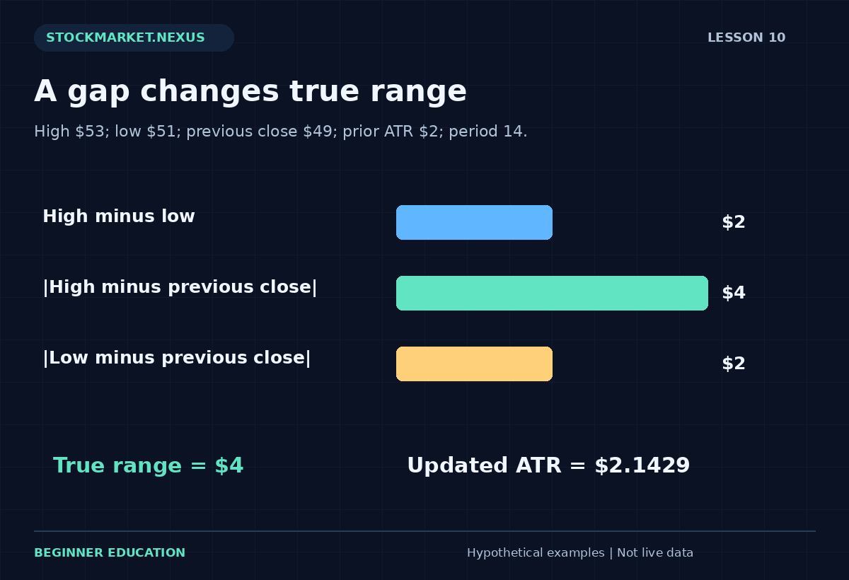
For high $53, low $51, previous close $49, the candidates are $2, $4, and $2. True range is $4. For high $49, low $47, previous close $52, the candidates are $2, $3, and $5, making true range $5. The formula includes the larger gap-aware distance rather than summing all distances.
If the previous close lies inside the new high-low interval, high minus low is the largest candidate. In that case true range equals the ordinary range. The additional comparisons matter when the previous close lies outside the new interval.
3. Update ATR from a prior state
This worksheet uses new ATR equal to prior ATR times period minus one, plus current true range, divided by period. If prior ATR is $2, period is 14, and current true range is $4, the new ATR is ($2 × 13 + $4) ÷ 14, approximately $2.1429.
The new large range raises the average but does not replace it. A longer period gives the prior state more weight in this update; a shorter period responds more quickly. Neither setting predicts the next range. They describe different smoothing choices applied to past observations.
A supplied prior ATR is essential for this one-step exercise. It does not construct the entire earlier series or verify the original seed. A full implementation needs an initialization convention and sufficient history. Different platforms can also use different smoothing choices, so reconcile definitions before comparing rounded values.
4. Keep units and scale visible
ATR is expressed in the same price units as the input series. An ATR of $2 has a different relative scale for a $20 instrument and a $200 instrument. A normalized comparison can divide ATR by a chosen reference price and multiply by 100, but that is an additional calculation with a stated denominator.
The worksheet reports ATR as a percentage of the supplied previous close. In the $49 previous-close example, new ATR about $2.1429 is approximately 4.37% of that reference. This is not a predicted daily percentage return and not a probability that tomorrow’s movement will be smaller.
A rising ATR can accompany a sharp advance, a sharp decline, or alternating large movements. The indicator measures magnitude rather than direction. Pairing it with a direction description is a separate analytical choice, not a property hidden inside the ATR value.
5. Understand why an average is not a boundary
An average of recent ranges does not cap future ranges. A new event can produce a movement several times larger than the selected ATR. A quiet historical sample can therefore coexist with substantial future gap risk. The average should not be presented as an insurance limit.
This distinction matters when learners use multiples of ATR for hypothetical exit distances. A two-ATR reference is a selected planning distance, not a guarantee that a fill will occur there or that the next move cannot exceed it. The order type, market conditions, and account exposure remain separate questions.
The technical levels and position risk lesson models a planned exit and a worse stressed exit separately. It illustrates why a precise chart distance can still produce an uncertain realized loss.
6. Compare ATR with other volatility descriptions
High-low range, standard deviation of closes, standard deviation of returns, and ATR summarize different inputs. They can change in different ways. A stock can have large intraday swings but finish near the same close repeatedly. Its true ranges can be substantial while close dispersion remains relatively modest.
Bollinger Bands in this course use the population standard deviation of a selected close window. The Bollinger Band lesson makes that convention explicit. A band-width reading and an ATR reading should not be expected to match numerically or carry identical interpretations.
Choose a measurement because it fits the research question. If the question concerns overnight discontinuities, a gap-aware range is relevant. If it concerns dispersion of closes around a mean, a different summary may be appropriate. More indicators do not automatically make the answer more reliable.
7. Work through the true-range worksheet
Open the Lesson 10 ATR exercise. Enter high 53, low 51, previous close 49, previous ATR 2, and period 14. Predict the three distances and the updated average before calculating. The result should show true range 4 and new ATR approximately 2.1429.
Change the previous close to 52 while keeping the high and low fixed. It now lies inside the bar, so true range becomes 2 and the ATR remains 2 under the supplied prior state. The change isolates the role of the gap without changing the current high-low range.
Next use high 49, low 47, and previous close 52. True range becomes 5. Try entering a high below the low; the worksheet should reject it. A previous ATR of zero is allowed as a supplied teaching state, but the tool does not claim it is a valid initialized history for a particular real instrument.
8. Inspect the graphic’s information limits
The exercise illustrates the current high-low interval and the previous-close reference. When the previous close falls outside the interval, the longer gap-aware distance becomes visible. The diagram does not imply that trades occurred continuously through every price between the old close and new interval.
A gap can leave no available transaction at a planned intermediate price. That operational reality is why a range measurement cannot guarantee execution. Review market, limit, and stop orders before assuming a chart threshold translates directly into a fill.
The visual also omits the order of intrabar movements. True range needs only high, low, and previous close, so it cannot tell which extreme occurred first. A backtest requiring that sequence needs additional data or an explicit conservative ambiguity rule.
9. Use a consistent volatility review process
Record the period, interval, smoothing convention, previous state, current true range, and normalized denominator if used. Compare like with like. A switch from daily to hourly bars changes the unit of observation; the resulting ATR is not simply a smaller version of the same statistic.
For a historical study, define whether ATR is measured before a signal or includes the signal bar. Using a completed signal bar’s large range to size an earlier hypothetical entry can introduce future information. The indicator timestamp should align with the actual decision time.
If a volatility filter is tested, preserve every eligible case and compare against a baseline. A rule that excludes quiet periods may also change exposure, turnover, and the distribution of event risk. A single improved average return does not describe all those changes.
10. Know what the number represents
You should be able to identify the three candidates, choose true range correctly for upward and downward gaps, update a supplied ATR, and distinguish price units from a normalized percentage. You should also explain why the indicator is directionless and why an average cannot guarantee an exit price.
ATR becomes useful when it improves the clarity of a question about observed movement. It becomes misleading when it is treated as a forecast, a fixed loss ceiling, or a substitute for execution planning. The calculation is simple; the professional skill is preserving those distinctions when applying it.
Case review: an unchanged range with a different prior close
High 53 and low 51 always create a $2 ordinary range. If the previous close is 52, true range is also $2. If the previous close is 49, true range becomes $4. The current bar’s geometry has not changed; the gap-aware reference has.
With supplied prior ATR 2 and period 14, the first case leaves ATR at 2, while the second raises it to about 2.1429. This isolates the contribution of the previous close and the smoothing state. It also shows why ATR is not simply an average of each bar’s high-low distance.
Write both cases side by side and label the previous close clearly. Do not draw a continuous trading path through the gap unless the data establishes one. The interval between a prior close and a later range can contain prices at which no included transaction occurred. That missing continuity matters for execution planning, even though the true-range formula can be calculated exactly from the supplied observations.
A repeatable practice and review protocol
Before changing the example, write down the question you expect the calculation to answer. Copy the input values, units, chronological order where relevant, and the observation time. State whether the values are fictional, historical, or current. The exercises in this course begin with fictional data so the arithmetic can be studied without implying that a real security offers a particular opportunity. A calculator result is only as meaningful as its input definitions.
Predict the direction of one change before pressing the calculation button. Change one input at a time, explain which part of the formula it affects, and compare the result with your prediction. This controlled approach is more informative than changing several fields until an attractive number appears. If the result surprises you, return to the definition and denominator before looking for a market explanation. Arithmetic mistakes and interpretation mistakes require different corrections.
Then test an ordinary alternative and an edge case. An ordinary alternative checks whether you understand the relationship away from the default example. An edge case checks whether a ratio becomes undefined, a sample becomes insufficient, or an input ordering becomes impossible. A clear validation message is a useful result. Do not work around it by entering an unrelated value merely to make the screen produce an answer. First understand which assumption the rejected value violated.
Save a short review with four parts: the observation, the calculation, the interpretation, and the unresolved limitation. Keep those parts separate. The observation records what the supplied data says; the calculation shows how the number was obtained; the interpretation is a conditional hypothesis; the limitation identifies information the exercise does not provide. This structure makes the note understandable to another beginner and makes later revisions easier to audit.
If you extend the example into a paper-trading study, define signal time, decision time, order assumptions, quantity, costs, and review horizon before checking the outcome. Preserve the original version. Record unfavorable cases and skipped cases under the same rules as favorable ones. A chart image can support the record, but it should not replace the actual values and definitions. A successful-looking historical picture is not a substitute for a complete sample.
Finish by explaining the result in plain language without using a pattern name as the explanation. Identify what changed, what stayed fixed, and what the exercise still cannot establish. You have completed the practice when you can reproduce the important arithmetic, recognize an invalid comparison, and describe an alternative outcome. Repeating this process across the course builds a consistent analytical habit while keeping the different formulas and their limitations distinct.
Sources and calculation notes
Primary educational background provides additional context for the topic. The fictional examples, teaching cases, diagrams, and worksheets here are original educational illustrations. Calculation conventions and missing information are stated explicitly; indicator readings do not establish future returns.