

Risk Management · Lesson 10 of 15 · Reviewed November 10, 2026
Different holdings can respond to the same event. A portfolio review should therefore ask what happens when several positions move adversely at once, including cases in which familiar offsets weaken. Joint stress testing makes those assumptions explicit without pretending to know their probability.
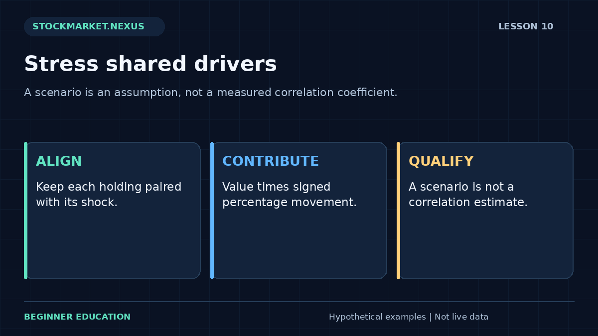
This lesson uses aligned position values and signed percentage shocks. The dedicated exercise calculates each scenario contribution, the portfolio change, and the post-shock value. It does not estimate a correlation coefficient or build a statistical risk model. The distinction between an assumed scenario and a measured historical relationship is central to the lesson.
1. Understand what correlation describes
Correlation summarizes a particular statistical relationship between aligned observations over a selected sample. It depends on the variables, interval, dates, and estimation method. A historical estimate is not a contractual promise about how two holdings will behave during the next event.
A price-level correlation can answer a different question from a return correlation. Different observation times, missing data, and currency effects can also distort the comparison. A credible statistical study needs definitions and data checks before interpreting a coefficient.
The worksheet avoids estimating one from insufficient inputs. A list of holding values and chosen shocks does not contain the return history required for that calculation. It is a scenario tool, and its output should be labeled accordingly.
2. Identify common economic drivers
Shared industry, financing conditions, geography, commodity exposure, or investor positioning can connect holdings that have different names. Fund overlap can create repeated issuer exposure. A stress review starts by describing these dependencies rather than assuming ticker variety creates independence.
Some dependencies are conditional. Holdings that behaved differently in ordinary periods may become more closely aligned under a liquidity event. That possibility does not prove they will always fall together; it supplies a reason to examine a common adverse case.
The concentration lesson measures value distribution and explains look-through overlap. Joint stress adds an explicit movement assumption for each included holding.

3. Apply signed shocks to aligned values
For each position, scenario dollar change equals current value times shock percentage divided by 100. Values 5000, 3000, 2000 with shocks −10%, −15%, and +2% produce changes −500, −450, and +40. Total change is −910.
The included portfolio begins at 10000 and ends at 9090, a 9.1% decline. The positive third contribution offsets part of the other losses under this chosen scenario. It is an assumption, not proof that the holding will provide that offset in a real event.
The lists must align by position. Applying one security’s shock to another security’s value produces a mathematically valid but analytically wrong result. Preserve labels and original assumptions in a separate record even when the exercise accepts only numerical lists.
4. Test the loss of an expected offset
Change the third shock from +2% to −5%. Its contribution becomes −100, so total change becomes −1050 and ending value 8950. The portfolio outcome worsens even though the first two assumptions remain fixed.
This controlled change is useful because it reveals how much the original conclusion depended on the offset. It does not require a claim that all correlations become one or that the new scenario is inevitable. Narrow scenario questions are often more defensible than dramatic universal statements.
A stress test should also explain why the chosen magnitudes are relevant to the study. Arbitrary numbers can teach arithmetic, as they do here, but they should not be presented as calibrated real-world risk limits or probabilities.
5. Distinguish a price shock from an executable exit
The post-shock value is a marked scenario under entered percentage changes. It is not necessarily the cash proceeds available from liquidating the positions. Spread, available quantity, halts, taxes, and execution timing can create differences.
A fully paid long holding cannot lose more than its value through price decline alone, so this exercise limits negative price shocks to −100%. Leverage, short positions, derivatives, and liabilities can create different exposure mechanics and are outside the long-value model.
The leverage lesson shows how debt changes the equity result. Do not apply a cash long-only scenario tool to a leveraged account without reconciling the missing liability structure.
6. Use the dedicated joint-stress exercise
Open the Lesson 10 joint-stress exercise. Enter values 5000, 3000, 2000 and shocks −10, −15, 2. Predict each contribution, total change minus 910, ending value 9090, and portfolio change minus 9.1%.
Change the final shock to −5 and explain the additional $140 deterioration. Then apply −10 to every position. The total declines 10%, illustrating that a common percentage shock carries through to the weighted portfolio when every included long value receives the same change.
Mismatched list lengths should produce an error. A total starting value of zero is also invalid for a percentage portfolio result. A zero-value holding can be included, but it contributes nothing and should not be mistaken for a meaningful diversifying allocation.
7. Compare several scenarios without assigning false precision
A useful review can include a broad market decline, a sector event, a liquidity deterioration, and an adverse offset case. Each scenario needs a clear purpose and a record of its assumptions. A table of precise outputs does not make the assumptions more certain.
Do not assign probabilities casually. A statement that a scenario has a 5% chance is a separate empirical or modeling claim requiring support. The exercise reports no probabilities, confidence levels, or value-at-risk estimate.
Keep favorable and unfavorable cases labeled symmetrically. Selecting only a stress in which one hedge works can create false reassurance. Selecting only an extreme collapse without explaining its purpose can create confusion rather than useful planning.
8. Connect scenarios with the account ledger
A portfolio shock should be considered alongside current equity, debt, planned open losses, available liquidity, and upcoming obligations. The same marked decline can have different practical consequences for accounts with different financing and cash needs.
The aggregate open-risk lesson compares loss-only planned and adverse amounts. This lesson uses signed percentage changes across current long values. Neither should be substituted silently for the other because their bases and conventions differ.
Record the valuation time and scenario version. If holdings change, rerun the calculation using the new weights. A stress result from last month does not describe a portfolio whose dominant holding has since doubled in size.
9. Case review: the hedge assumption carries the conclusion
A fictional review reports that two risky holdings lose $950 while a third gains $800, leaving a modest $150 net decline. The arithmetic can be correct, but the conclusion depends heavily on the third contribution. If that contribution is uncertain or based on a different event regime, the apparent protection deserves scrutiny.
A second scenario holds the first two losses fixed and sets the third contribution to zero. A third makes it negative. The comparison shows the sensitivity without claiming which case will occur. This is a more useful discussion than calling the portfolio hedged without qualification.
For practice, identify the largest favorable contribution in a scenario and ask what evidence supports it. Then remove or reverse that assumption in a separate case. The goal is to understand dependencies and limits, not to create a dramatic forecast or certify that a portfolio can survive every event.
Review challenge: the same total hides different contributions
Consider two $10,000 portfolios with the same minus $900 scenario total. In one, every holding declines moderately. In the other, one holding loses $2,000 while another gains $1,100. The net total matches, but the dependence on the favorable offset differs.
A contribution chart makes that distinction visible. It does not prove the offset will fail, but it identifies an assumption worth testing separately. Hold the adverse contribution fixed and reduce the favorable one to zero in a new case. The change reveals how much of the original conclusion depended on it.
Do not label that experiment a measured change in correlation. No historical return sample was estimated. It is a scenario sensitivity test with explicit signed shocks. The distinction matters because a statistical term can make a chosen assumption sound more empirical than it is.
For practice, record the starting values, aligned shock list, contribution amounts, and rationale for each case. State that the post-shock values are marks rather than guaranteed liquidation proceeds. This keeps the analysis useful without turning a simple weighted calculation into a probability model or a promise that a hedge will offset losses when it is needed.
A complete practice record: assumptions, calculation, and review
Start the exercise by copying its inputs into a short record before pressing Calculate. Identify every unit and denominator: dollars, shares, percentages, price units, or a count of completed observations. Write the valuation time and clarify whether the values are fictional, historical, or confirmed transactions. The defaults in this course are fictional teaching examples. Their purpose is to make the arithmetic reproducible, not to recommend a position, percentage, boundary, or financing arrangement for a particular person.
Name the assumption that has the greatest effect on the answer. In one exercise it may be an exit fill; in another it may be the portfolio value, a shared shock, a cost, or the definition of the risk unit. A precise result can be highly sensitive to one uncertain input. State that sensitivity in plain language rather than allowing a clean screen to imply certainty. The calculator can enforce numerical consistency, but it cannot verify that the source data or chosen policy fits a real account.
Predict the result of one controlled change before calculating again. Keep every other input fixed. Explain whether the change affects a numerator, denominator, quantity constraint, cost, or scenario branch. Then compare the displayed result with your prediction. If they differ, return to the definition and arithmetic before inventing a market explanation. This method teaches the relationship among the inputs and prevents experimentation from becoming a search for a reassuring output.
Test a boundary case deliberately. Ask what happens when no whole share fits, a denominator becomes zero, a list is incomplete, a quantity exceeds the holding, or a scenario no longer matches the required price ordering. A validation message is useful evidence about the model’s scope. Do not replace a rejected value with an unrelated number simply to obtain an answer. First identify the violated assumption and decide whether this exercise is the appropriate model for the question.
Keep intended actions separate from confirmed states. A submitted order is not a completed fill, a cancellation request is not necessarily a canceled instruction, and a chart reference is not an available transaction price. For a paper exercise, state the hypothetical execution assumption. For a completed transaction record, use actual quantities, prices, charges, and status. Reconcile partial fills and remaining instructions so the ledger describes the exposure that exists rather than the exposure that was intended.
Write both the ordinary scenario and an adverse alternative when the model permits it. Preserve the original quantity while testing a worse outcome unless the purpose is explicitly to design a new plan. Label any revised plan with its own time and assumptions. A stress case is one selected possibility; it is not automatically the worst conceivable outcome or an estimate of probability. Missing information should remain labeled as missing rather than being converted into a zero or a favorable assumption.
Review the result on two separate dimensions. The first is outcome: what net dollars or normalized result occurred under the stated convention? The second is process: were the original definitions, constraints, and reconciliation steps followed? A favorable outcome does not prove a deviation was sound, and a loss does not prove that correct arithmetic was wrong. This separation helps a beginner identify a specific improvement instead of responding to every result with a new rule.
Finish with a concise explanation containing the observation, calculation, interpretation, and limitation. Another reader should be able to reproduce the important numbers without guessing what the fields mean. Preserve the original record, later revisions, and unfavorable examples. If extending the exercise into a historical or forward paper study, define the eligible sample and review horizon before collecting outcomes. A selected group of attractive examples cannot establish the reliability of a process. The strongest learning result is a clearer, auditable decision routine, including a clear reason when an example remains unresolved or does not fit the entered constraints.
Sources and model scope
Primary investor-education background supplies additional context. The numerical cases, graphics, and worksheets here are original fictional teaching examples. Every calculation depends on its stated convention; no worksheet determines personal suitability, guarantees execution, or establishes future returns.