

Risk Management · Lesson 11 of 15 · Reviewed November 10, 2026
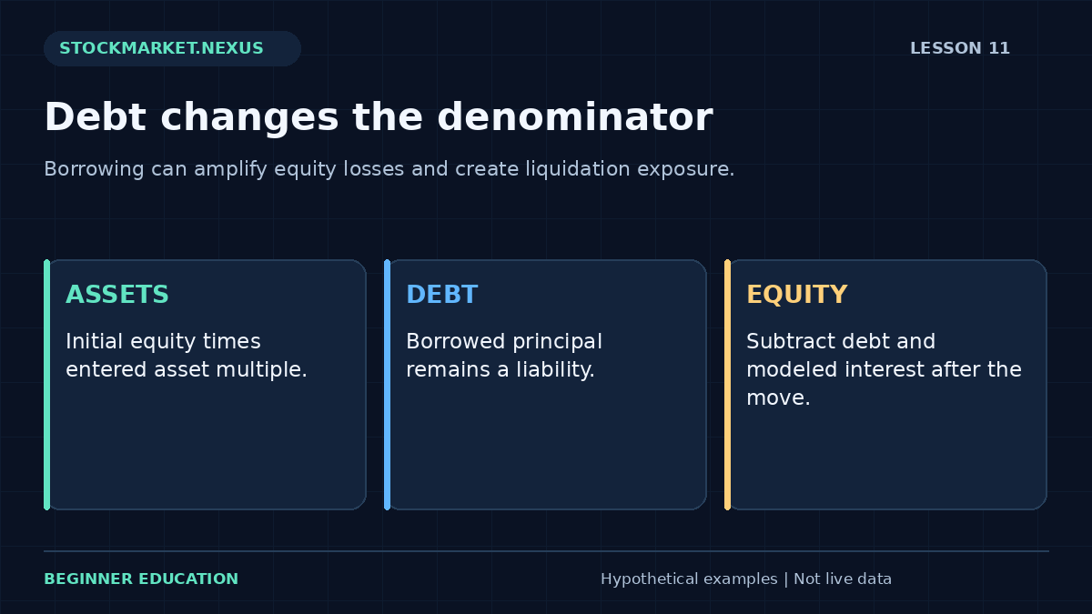
Borrowing can make the percentage change in account equity larger than the percentage change in the purchased assets. The mechanism is straightforward: asset value changes while the debt remains owed, and financing costs can add to the liability. A professional explanation traces each balance rather than presenting leverage as extra buying power without its downside.
This lesson uses a simplified financed long-position scenario. The exercise calculates initial assets, debt, post-move assets, simple interest, ending equity, and equity return. It does not determine margin eligibility, regulatory requirements, broker house rules, maintenance thresholds, or the timing of any liquidation.
1. Begin with the balance-sheet identity
Equity equals assets minus liabilities. If a fictional account contributes $5,000 and borrows $5,000 to buy $10,000 of assets, initial equity is $5,000. Gross asset exposure is twice that equity under the exercise’s asset-multiple convention.
The multiple describes the entered starting structure. It is not a promise that a broker will provide that financing or permit it to remain open. Actual account permissions and requirements depend on the product, service, agreement, and applicable rules.
The risk-ledger lesson separates capital and exposure. Leverage adds a liability that must remain visible in the denominator and scenario calculation.
2. Calculate the asset-price effect
A 10% decline in $10,000 of assets reduces them to $9,000. Before interest, the $5,000 debt remains, leaving $4,000 equity. The asset decline is 10%, while the equity decline is 20% from the original $5,000 contribution.
A 10% asset gain raises assets to $11,000 and equity to $6,000 before interest, a 20% equity gain. The amplification works in both directions under this simplified structure. It does not create a favorable expected return by itself.
If assets fall far enough, equity can reach zero or become negative relative to the debt. The exercise displays negative scenario equity rather than flooring it to zero, because the liability does not disappear when the asset value declines.

3. Include a transparent interest convention
The worksheet estimates simple interest as debt times annual rate times days divided by 365. With $5,000 debt, annual rate 10%, and 30 days, modeled interest is about $41.10. Subtracting it from the $4,000 post-decline equity leaves about $3,958.90.
The resulting equity return is approximately −20.82% from the original $5,000. This convention is an educational approximation. Actual interest can depend on changing balances, tiered rates, day-count conventions, compounding, and account terms.
Do not count the borrowed principal as a cost that disappears after purchase or as equity contributed by the account owner. It is a liability that remains part of the closing balance-sheet calculation. Interest is a separate financing charge.
4. Recognize liquidation and requirement uncertainty
A broker can impose maintenance and house requirements and may liquidate positions under the account agreement. Requirements can change, and a simplified price-shock worksheet does not establish the point at which a real account would receive a call or be liquidated.
The exercise deliberately avoids a “safe until this price” output. Such a claim would need current product-specific and broker-specific information, including how the whole account is margined. One isolated asset multiple is not enough.
Review the broker’s current agreement and requirements for any real account. This lesson explains the balance-sheet mechanics without substituting a generic percentage for those operational terms.
5. Distinguish leverage from position allocation
A fully paid $5,000 holding inside a $10,000 account has a 50% allocation but does not require borrowing under that scenario. A $10,000 holding financed with $5,000 equity and $5,000 debt has different exposure mechanics. Similar position values can therefore imply different equity risk.
Derivatives and leveraged funds introduce additional structures that this model does not capture. A fund’s stated daily objective is not the same as a static margin loan, and option obligations are not fully described by asset value minus one debt balance.
The concentration lesson also remains relevant. Borrowing against a concentrated exposure can combine amplification with dependence on one driver. A leverage number alone does not describe the whole portfolio.
6. Use the dedicated leverage exercise
Open the Lesson 11 leverage exercise. Enter initial equity 5000, asset multiple 2, asset move −10%, annual interest rate 10%, and days 30. Predict assets 10000, debt 5000, post-move assets 9000, interest about 41.10, and ending equity about 3958.90.
Change the asset move to +10%. The financing cost remains while the asset result changes sign. Next reduce the multiple to one. Debt becomes zero and modeled interest becomes zero, isolating the effect of borrowing under this convention.
Try an asset decline of 60% with multiple two. Assets become $4,000 before costs while debt remains $5,000, producing negative equity even before interest. The worksheet does not claim a real broker would allow the position to remain untouched through that path; it shows the liability arithmetic of the selected endpoint.
7. Understand the denominator after losses
As equity falls, the same remaining asset value can represent a larger exposure multiple. In the initial example, $9,000 assets divided by $4,000 equity is 2.25 before interest, higher than the starting multiple of two. Exposure can become more concentrated relative to equity without a new purchase.
A later reduction in assets, repayment, or liquidation would change the path. The endpoint worksheet does not simulate those actions. A complete account model would need ordered events and current requirements rather than a single price move.
The drawdown lesson explains why recovery percentages grow as the equity base shrinks. Borrowing can make that shrinking base more consequential.
8. Avoid treating buying power as loss-absorbing capital
An available purchasing limit is not the same as cash the account can afford to lose. It can change with prices, requirements, and account state. A plan that uses the maximum available amount without tracing liabilities can confuse permission with capacity.
A risk review should identify the source of equity, financing costs, liquidity needs, concentration, and adverse scenarios. The worksheet does not collect that personal context or recommend a multiple. Its fictional defaults exist to demonstrate the formula.
Keep actual loan balances and charges in the ledger. A favorable market move does not make financing free, and a loss does not cancel the repayment obligation. These basic accounting distinctions are the foundation of a professional leverage explanation.
9. Case review: the same asset loss, different equity loss
Compare a fully paid $5,000 asset holding with a $10,000 holding financed by $5,000 equity and $5,000 debt. A 10% asset decline costs the first $500 and the second $1,000 before financing. Both owners began with $5,000 equity, so their equity changes differ materially.
The second example also incurs interest under the chosen convention. If a review reports only the common 10% market decline, it omits the financing structure that determines the account result. If it reports only the larger initial asset value, it omits the debt.
For practice, draw a three-line ledger for assets, liabilities, and equity before and after the shock. Add interest separately. Explain why the model cannot certify a margin-call threshold. The professional objective is to make the mechanism and missing account-specific information visible, not to encourage borrowing or present a universal leverage rule.
Review challenge: financing continues while the asset pauses
Use equity $4,000, asset multiple 1.5, annual interest 12%, and 60 days. Starting assets are $6,000 and debt $2,000. If asset price is unchanged, simple modeled interest is about $39.45, leaving equity about $3,960.55. A flat asset price does not imply a flat equity result when financing costs accrue.
Now apply a 20% asset decline. Assets become $4,800, while debt and the modeled interest remain. Ending equity is about $2,760.55, a much larger percentage decline than the asset’s 20%. The liability and denominator explain the difference.
This endpoint does not establish when a real broker would intervene or whether the position could remain open for the full 60 days. Requirements, other holdings, and account terms are missing. A professional model states that limitation instead of producing a generic margin-call price.
For practice, reconcile the three-line balance sheet before and after the scenario. Then calculate interest separately and check that it is not deducted twice. Keep initial equity, asset exposure, debt, and ending equity distinct. The borrowing capacity shown by a service is not the same thing as loss-absorbing personal capital, and the exercise does not decide an appropriate leverage level.
A complete practice record: assumptions, calculation, and review
Start the exercise by copying its inputs into a short record before pressing Calculate. Identify every unit and denominator: dollars, shares, percentages, price units, or a count of completed observations. Write the valuation time and clarify whether the values are fictional, historical, or confirmed transactions. The defaults in this course are fictional teaching examples. Their purpose is to make the arithmetic reproducible, not to recommend a position, percentage, boundary, or financing arrangement for a particular person.
Name the assumption that has the greatest effect on the answer. In one exercise it may be an exit fill; in another it may be the portfolio value, a shared shock, a cost, or the definition of the risk unit. A precise result can be highly sensitive to one uncertain input. State that sensitivity in plain language rather than allowing a clean screen to imply certainty. The calculator can enforce numerical consistency, but it cannot verify that the source data or chosen policy fits a real account.
Predict the result of one controlled change before calculating again. Keep every other input fixed. Explain whether the change affects a numerator, denominator, quantity constraint, cost, or scenario branch. Then compare the displayed result with your prediction. If they differ, return to the definition and arithmetic before inventing a market explanation. This method teaches the relationship among the inputs and prevents experimentation from becoming a search for a reassuring output.
Test a boundary case deliberately. Ask what happens when no whole share fits, a denominator becomes zero, a list is incomplete, a quantity exceeds the holding, or a scenario no longer matches the required price ordering. A validation message is useful evidence about the model’s scope. Do not replace a rejected value with an unrelated number simply to obtain an answer. First identify the violated assumption and decide whether this exercise is the appropriate model for the question.
Keep intended actions separate from confirmed states. A submitted order is not a completed fill, a cancellation request is not necessarily a canceled instruction, and a chart reference is not an available transaction price. For a paper exercise, state the hypothetical execution assumption. For a completed transaction record, use actual quantities, prices, charges, and status. Reconcile partial fills and remaining instructions so the ledger describes the exposure that exists rather than the exposure that was intended.
Write both the ordinary scenario and an adverse alternative when the model permits it. Preserve the original quantity while testing a worse outcome unless the purpose is explicitly to design a new plan. Label any revised plan with its own time and assumptions. A stress case is one selected possibility; it is not automatically the worst conceivable outcome or an estimate of probability. Missing information should remain labeled as missing rather than being converted into a zero or a favorable assumption.
Review the result on two separate dimensions. The first is outcome: what net dollars or normalized result occurred under the stated convention? The second is process: were the original definitions, constraints, and reconciliation steps followed? A favorable outcome does not prove a deviation was sound, and a loss does not prove that correct arithmetic was wrong. This separation helps a beginner identify a specific improvement instead of responding to every result with a new rule.
Finish with a concise explanation containing the observation, calculation, interpretation, and limitation. Another reader should be able to reproduce the important numbers without guessing what the fields mean. Preserve the original record, later revisions, and unfavorable examples. If extending the exercise into a historical or forward paper study, define the eligible sample and review horizon before collecting outcomes. A selected group of attractive examples cannot establish the reliability of a process. The strongest learning result is a clearer, auditable decision routine, including a clear reason when an example remains unresolved or does not fit the entered constraints.
Sources and model scope
Primary investor-education background supplies additional context. The numerical cases, graphics, and worksheets here are original fictional teaching examples. Every calculation depends on its stated convention; no worksheet determines personal suitability, guarantees execution, or establishes future returns.