


Risk Management · Lesson 04 of 15 · Reviewed November 10, 2026
A large target relative to a planned loss can make a trade diagram attractive, but the ratio alone does not establish positive expected value. The chance of each outcome, execution costs, actual outcome sizes, and failures outside the simplified model all matter. Risk management requires keeping those concepts separate.
This lesson distinguishes planned price geometry from a probability-weighted scenario. The dedicated exercise accepts an assumed win rate, average gross gain, average gross loss magnitude, and fixed cost per trade. It calculates the consequences of those assumptions without estimating a real win probability or recommending a strategy.
1. Define the ratio being reported
A gross reward-to-risk ratio divides a selected potential gain by a selected potential loss. If the scenario gain is $200 and loss magnitude $100, the ratio is 2.0. This does not mean the gain is twice as likely, that two gains will occur for every loss, or that a target will be reached before a protective reference.
The selected target can be moved farther away to increase the ratio on paper. The exit reference can be tightened to create the same effect. Neither adjustment proves the new outcome is more attainable or operationally coherent. A ratio is meaningful only alongside the hypothesis and execution assumptions that produced its inputs.
The technical-level planning lesson demonstrates price-distance geometry. Here the focus shifts to the outcome distribution and the effect of costs.
2. Calculate an assumed expected value
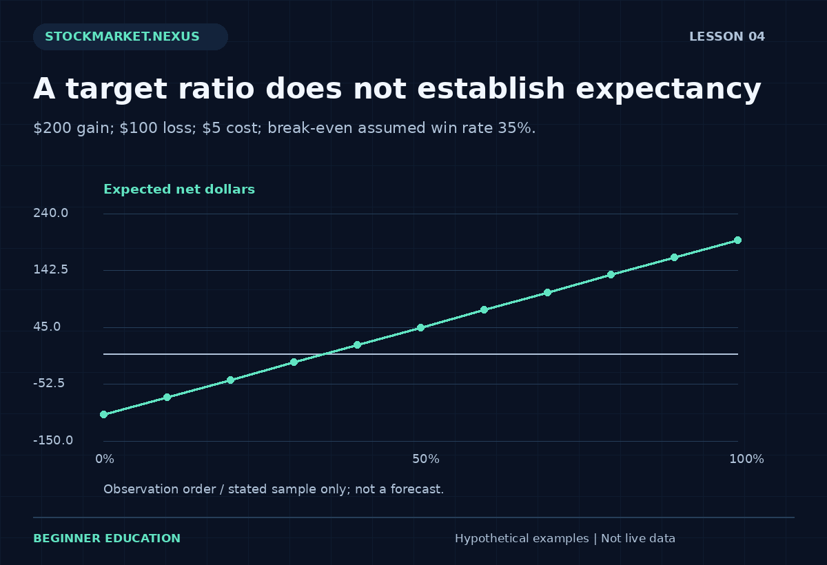
Under a simplified two-outcome model, expected net result equals assumed win fraction times average gross gain, minus loss fraction times average gross loss magnitude, minus fixed cost per trade. The loss fraction is one minus the win fraction. The average outcomes are positive magnitudes; the subtraction supplies the loss sign.
With assumed win rate 40%, gain $200, loss $100, and cost $5, expected net result is 0.40 × $200 − 0.60 × $100 − $5 = $15 per trade. This is the mathematical expectation of the entered model, not a forecast that the next trade will make $15.
The expectation depends entirely on the supplied assumptions. If the win rate was guessed or selected from an optimistic sample, the output does not repair that weakness. A precise result can still rest on an uncertain probability.
3. Include costs in both outcome branches
A gross winner of $200 becomes a net winner of $195 after the $5 cost. A gross loser of $100 becomes a net loser of $105. The equivalent expectation is 0.40 × $195 − 0.60 × $105 = $15. Showing both branches makes it clear that charges apply regardless of direction.
If costs vary with quantity, liquidity, or holding period, one fixed input is only an approximation. Financing, borrowing, taxes, and unusual execution events may require additional fields. A beginner should identify the convention before comparing reported results from different studies.
Costs can also change which gross outcomes remain net winners. A very small gross gain can become a net loss. A sample labeled by gross outcomes should retain that distinction rather than presenting gross win rate as though it were the net winning frequency.
4. Derive the simplified break-even win rate
Setting the expected net result to zero gives break-even win fraction equal to loss magnitude plus cost, divided by gain plus loss magnitude. For gain $200, loss $100, and cost $5, the threshold is 105/300, or 35%.
This threshold assumes the average gains, average losses, and fixed costs remain as entered. It does not estimate how often the strategy actually wins. A method with a 35% arithmetic threshold can still perform poorly if its real gain distribution, costs, or failure scenarios differ.
If the cost exceeds the gross gain, the required fraction can exceed 100%. That result is not a bug: it reveals that the simplified economics cannot break even through win frequency alone under the supplied values. The tool should label the infeasible threshold rather than cap it at a reassuring number.
5. Distinguish expectation from path risk
Two sequences can have the same average outcome and very different drawdowns. Several losses early in a sample can create a difficult capital path even when later gains produce a positive final total. Expectation alone does not describe the order of events, largest loss, or capital needed to continue.
An average also hides tail outcomes. A model with a fixed $100 loss excludes any larger adverse event by construction. If gaps can create occasional $400 losses, those outcomes belong in a richer distribution or a separate stress scenario. They should not disappear because a two-outcome worksheet is convenient.
The losing-streak lesson explores deterministic sequences without pretending to calculate their probability. The distinction between average economics and sequence exposure is essential to a complete review.
6. Use the dedicated expectancy exercise
Open the Lesson 4 expectancy exercise. Enter assumed win rate 40, gross gain 200, gross loss 100, and cost 5. Predict gross ratio 2, net winning outcome 195, net losing magnitude 105, expected net result 15, and break-even rate 35%.
Reduce the assumed win rate to 30%. Expected net result becomes $60 − $70 − $5 = −$15. The target-loss ratio remains 2.0. This isolates why a favorable-looking ratio does not settle the economic question.
Next restore 40% and raise cost to $25. Expected result becomes negative $5. A changing cost assumption can reverse the conclusion even when the outcome sizes and assumed frequency stay fixed. The exercise is successful when you can explain that sensitivity before reading the output.
7. Avoid treating a historical frequency as a known probability
A small sample’s winning fraction is an observation, not a stable probability supplied by the market. Selection, changing conditions, overlapping trades, and parameter searches can all affect how representative the sample is. The worksheet does not calculate confidence intervals or independence tests.
A historical strategy study should preserve eligible cases, execution assumptions, and all tested versions. Repeatedly choosing the settings with the best observed frequency can fit noise. A later independent evaluation is needed before making stronger claims about durability.
Review backtesting technical strategies for the difference between sample arithmetic and evidence of an edge. The expectancy exercise is one audit component within that broader process.
8. Report the result with its assumptions
A useful statement says, “Under a 40% assumed winning frequency, $200 average gross gain, $100 average gross loss, and $5 fixed cost, the two-outcome expectation is $15.” This is narrower and more accurate than saying the strategy earns $15 per trade.
Also state which outcomes are omitted. Breakeven trades, variable quantities, partial exits, rare losses, and changing costs can all require a more detailed ledger. A simple model is useful when its scope is clear and dangerous when its omissions are hidden.
Do not interpret a positive output as an instruction to increase size. Quantity changes can alter costs, liquidity, and the distribution itself. The model’s inputs are assumptions to examine, not permissions granted by the calculator.
9. Case review: a better ratio with worse expectation
Compare model A with gain $200, loss $100, 40% assumed wins, and $5 cost against model B with gain $400, loss $100, 15% assumed wins, and the same cost. A has ratio 2 and expectation $15. B has ratio 4 but expectation $60 − $85 − $5 = −$30.
The larger ratio does not make B economically superior under these assumptions. Its lower winning frequency more than offsets the larger favorable outcome. This is a mathematical comparison, not evidence that a real wider target would have exactly that frequency.
For practice, write the assumptions beneath each model and identify which were measured, estimated, or merely chosen. The most important uncertainty may be the input frequency rather than the arithmetic. A professional review makes that uncertainty visible instead of allowing a large target multiple to dominate the discussion.
Review challenge: assumptions dominate the expectation
Take gross gain $120, loss magnitude $80, and fixed cost $4. The simplified break-even win rate is $84/$200, or 42%. At an assumed 50% winning frequency, expected net result is $60 minus $40 minus $4, or $16. At an assumed 40%, it becomes $48 minus $48 minus $4, or minus $4.
The arithmetic changes sharply even though the gross ratio remains 1.5. A learner should therefore identify how the winning-frequency input was obtained. A guess, a selected chart collection, and a complete predefined sample do not provide the same evidential support.
Next keep the frequency at 50% and change average loss to $120. Expected net result becomes minus $4. This demonstrates that an optimistic loss magnitude can matter as much as an optimistic frequency. Rare adverse fills can change the relevant average and the shape of the distribution.
For the record, label each input as observed, estimated, or chosen for teaching. Do not allow a positive calculated expectation to upgrade uncertain inputs into facts. A professional explanation preserves the conditional statement and asks which additional data would be needed to evaluate whether the model represents actual outcomes. The worksheet performs arithmetic, while the research process must justify the assumptions.
A complete practice record: assumptions, calculation, and review
Start the exercise by copying its inputs into a short record before pressing Calculate. Identify every unit and denominator: dollars, shares, percentages, price units, or a count of completed observations. Write the valuation time and clarify whether the values are fictional, historical, or confirmed transactions. The defaults in this course are fictional teaching examples. Their purpose is to make the arithmetic reproducible, not to recommend a position, percentage, boundary, or financing arrangement for a particular person.
Name the assumption that has the greatest effect on the answer. In one exercise it may be an exit fill; in another it may be the portfolio value, a shared shock, a cost, or the definition of the risk unit. A precise result can be highly sensitive to one uncertain input. State that sensitivity in plain language rather than allowing a clean screen to imply certainty. The calculator can enforce numerical consistency, but it cannot verify that the source data or chosen policy fits a real account.
Predict the result of one controlled change before calculating again. Keep every other input fixed. Explain whether the change affects a numerator, denominator, quantity constraint, cost, or scenario branch. Then compare the displayed result with your prediction. If they differ, return to the definition and arithmetic before inventing a market explanation. This method teaches the relationship among the inputs and prevents experimentation from becoming a search for a reassuring output.
Test a boundary case deliberately. Ask what happens when no whole share fits, a denominator becomes zero, a list is incomplete, a quantity exceeds the holding, or a scenario no longer matches the required price ordering. A validation message is useful evidence about the model’s scope. Do not replace a rejected value with an unrelated number simply to obtain an answer. First identify the violated assumption and decide whether this exercise is the appropriate model for the question.
Keep intended actions separate from confirmed states. A submitted order is not a completed fill, a cancellation request is not necessarily a canceled instruction, and a chart reference is not an available transaction price. For a paper exercise, state the hypothetical execution assumption. For a completed transaction record, use actual quantities, prices, charges, and status. Reconcile partial fills and remaining instructions so the ledger describes the exposure that exists rather than the exposure that was intended.
Write both the ordinary scenario and an adverse alternative when the model permits it. Preserve the original quantity while testing a worse outcome unless the purpose is explicitly to design a new plan. Label any revised plan with its own time and assumptions. A stress case is one selected possibility; it is not automatically the worst conceivable outcome or an estimate of probability. Missing information should remain labeled as missing rather than being converted into a zero or a favorable assumption.
Review the result on two separate dimensions. The first is outcome: what net dollars or normalized result occurred under the stated convention? The second is process: were the original definitions, constraints, and reconciliation steps followed? A favorable outcome does not prove a deviation was sound, and a loss does not prove that correct arithmetic was wrong. This separation helps a beginner identify a specific improvement instead of responding to every result with a new rule.
Finish with a concise explanation containing the observation, calculation, interpretation, and limitation. Another reader should be able to reproduce the important numbers without guessing what the fields mean. Preserve the original record, later revisions, and unfavorable examples. If extending the exercise into a historical or forward paper study, define the eligible sample and review horizon before collecting outcomes. A selected group of attractive examples cannot establish the reliability of a process. The strongest learning result is a clearer, auditable decision routine, including a clear reason when an example remains unresolved or does not fit the entered constraints.
Sources and model scope
Primary investor-education background supplies additional context. The numerical cases, graphics, and worksheets here are original fictional teaching examples. Every calculation depends on its stated convention; no worksheet determines personal suitability, guarantees execution, or establishes future returns.