

Options Trading · Lesson 14 of 15 · Reviewed November 10, 2026
A credit vertical spread sells one option and buys another of the same type and expiration on the same underlying, using different strikes and a net premium receipt. The long leg changes the theoretical expiration exposure, but the short leg still creates an obligation. Receiving a credit is not proof that the position is low risk.
This lesson uses standard one-for-one bull put and bear call examples with a 100 multiplier. The expiration boundaries assume matching terms and an intact structure. Account events such as early assignment, unmatched exercise, separate-leg execution, or broker liquidation require additional operational analysis.
1. Define a bull put spread
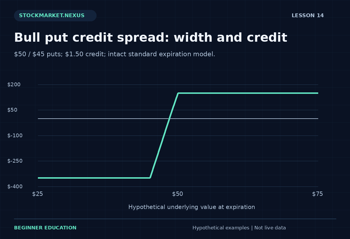
A bull put spread sells a higher-strike put and buys a lower-strike put with the same expiration. Consider a fictional short $50 put and long $45 put for a $1.50 net credit per share. The width is $5, and the initial premium receipt is $150 per standard spread before charges.
The favorable expiration region is at or above the higher strike, where the simplified intrinsic obligation is zero. Below the lower strike, the long put offsets further widening of the intrinsic difference in the intact model. The credit limits the favorable outcome but does not prevent a larger adverse result.
The cash-secured-put lesson explains the short put obligation. Adding the lower-strike long put changes the theoretical structure, but it does not make the short contract cease to exist as a separately assignable position.
2. Calculate bull put expiration economics
Maximum modeled gain is the $150 credit per standard spread before charges. Maximum modeled loss is $350: width minus credit, multiplied by 100. Breakeven is $48.50, the short put strike minus credit.
At an underlying value of $55, the model retains the $150. At $48, the spread's intrinsic obligation is $2 per share, exceeding the $1.50 credit by fifty cents and producing a $50 loss. At $40, the intrinsic difference reaches the $5 width and the modeled result is minus $350.
The ratio of maximum gain to maximum loss does not establish the probability of either. A high fraction of profitable examples can coexist with a negative net result if losses, charges, or management behavior dominate. Report actual outcomes rather than converting a credit amount into a promised recurring return.
3. Define a bear call spread
A bear call spread sells a lower-strike call and buys a higher-strike call with the same expiration. A fictional short $50 call and long $55 call for a $1.50 credit also has a $5 width. Its favorable expiration region is at or below $50.
Maximum modeled gain is $150 and maximum modeled loss $350 before charges. Breakeven is $51.50, the short call strike plus credit. At $52, the $2 intrinsic difference creates a $50 loss after credit. At $60, the width caps the intrinsic difference in the intact expiration model.
The debit-spread lesson provides a useful comparison of signed legs and initial cash flows. Different credits, debits, and strikes should not be compared without consistent contract terms and execution assumptions.
4. Evaluate collateral and resources separately
A broker's displayed buying-power requirement depends on account rules and the recognized structure. It is not automatically identical to every adverse account-state requirement after assignment. Verify the actual agreement and the treatment of the spread before assuming that a width-based worksheet describes all necessary resources.
If one leg is assigned and the other remains open, the account can contain shares and an option rather than the original two-option structure. Price changes and financing can matter during that interval. The theoretical expiration cap does not submit an offsetting instruction or guarantee its execution.
The exercise and assignment lesson explains why the account transition must be planned. A defined-risk label should introduce the assumptions of a model, not end the discussion of operational exposure.
5. Treat closing cost and rolling credits honestly
Buying back a credit spread can cost more than the opening credit. The realized result is credit received minus debit paid to close, scaled by multiplier and quantity, less charges. A remaining open position should not be reported as having earned the entire credit merely because the cash arrived initially.
A roll closes the old structure and opens a new one. Preserve the old realized result, the new credit or debit, and the new obligations. Extending expiration can change event exposure and resources. A net-credit roll does not prove that the original loss vanished.
Multi-leg instructions can express a desired net limit, but a fill is not guaranteed. If the account uses separate-leg execution, the temporary position can differ substantially from the intended spread. The journal should record what actually existed rather than only the final strategy name.
6. Practice favorable, middle, and adverse regions
Use the credit-spread exercise to choose bull put or bear call, strikes, credit, quantity, and a hypothetical terminal value. The worksheet should reject a credit outside the coherent width range of its simplified model.
Compare both strikes and the breakeven. Include a point between strikes where the position loses less than the modeled maximum, rather than teaching only all-or-nothing outcomes. Add explicit charges consistently to show how they reduce gains and increase losses.
Finally, describe a one-leg assignment scenario in words. The numerical payoff table and the operational plan serve different purposes. A professional lesson should allow the visitor to understand both without suggesting that a clean maximum-loss number removes the need for account monitoring.
## Worked bull put spread across the strike interval
Use a short $50 put and long $45 put entered for a $1.50 credit. At terminal underlying values of $55, $48, and $40, the short-put intrinsic obligations are zero, $2, and $10. The long-put intrinsic values are zero, zero, and $5. Net obligations are zero, $2, and $5 per share.
The premium credit produces results of plus $150, minus $50, and minus $350 per standard spread before charges. The middle row demonstrates a partial loss rather than an all-or-nothing outcome. A simplified diagram should include that region so learners understand how the payoff changes between strikes.
With a fictional $4 total charge, maximum modeled gain becomes $146 and maximum modeled loss becomes $354. Breakeven rises from $48.50 to $48.54 when interpreted as the underlying value needed to avoid a loss in the put spread's middle region. More precisely, the cost-adjusted credit is $1.46, so the required value is $50 minus $1.46. Keep the arithmetic explicit to avoid a directional sign mistake.
Worked bear call spread with mirrored direction
Use a short $50 call and long $55 call for the same $1.50 credit. At underlying values of $45, $52, and $60, net intrinsic obligations are zero, $2, and $5. Results are plus $150, minus $50, and minus $350 before charges, with the favorable region on the lower-price side.
The uncharged breakeven is $51.50. With a $4 total charge for one standard spread, the effective credit is $1.46 per share and the cost-adjusted breakeven becomes $51.46. Charges reduce the favorable room rather than changing the contract strikes.
These mirrored examples are a useful sign check. A bullish put spread and bearish call spread can share width and credit while responding in opposite directions. The worksheet must name type, long strike, short strike, and position signs, not only the opening cash flow.
Compare credit collected with a completed trade result
If a spread opens for a $1.50 credit and later closes for a $2.20 debit, the premium result is minus seventy cents per share, or minus $70 per standard spread before charges. The original $150 receipt was a cash flow, not a guaranteed final gain.
If a roll then opens another spread for a $2.50 credit, the new receipt does not erase the old loss. The journal should retain the closure and new opening separately. The replacement has another expiration, event window, and set of obligations, even if the ticket displays a net credit.
A series of profitable-looking credits can therefore coexist with a negative account result. Evaluate realized and open positions under a consistent convention. Do not report only premium received while omitting buybacks, stock transitions, or charges that materially change the total.
Keep width-based exposure within its model scope
The intact spread's theoretical expiration loss is based on the strike width and credit under matching terms. That calculation does not guarantee every temporary account state after early assignment or uneven expiration processing. A short leg can create stock while the long leg remains an option.
The account may need resources or another verified action to manage that state. The long contract is not an automatic account administrator. A professional practice exercise should explain the exception even when its calculator intentionally models only the intact terminal payoff.
Finish by writing the plan for closure and the procedure for an unfilled closing instruction. A risk boundary on a diagram is useful only when the learner also understands what is currently held, what remains owed, and what confirmation is required before the position is considered gone.
## How to complete and review the lesson exercise
Start by writing the contract identity and the calculation's time horizon before entering numbers. A quoted premium, a hypothetical expiration value, and a strike-related cash transaction are different inputs. State which one the exercise uses. This prevents a correct arithmetic operation from answering the wrong question. The worksheet should support the lesson's definitions rather than encourage the visitor to infer a real trade from an attractive output.
Next, translate every per-share figure into the stated contract units. Use the actual multiplier and deliverable when studying a real specification; the lesson exercises intentionally use clearly labeled standard examples. Keep quantity separate from price. Increasing contract count changes total dollars and obligations without improving the underlying hypothesis. A small premium displayed on a chain can therefore become a material aggregate amount when multiplied across several contracts.
Use three input checks before interpreting the result. First, confirm that the option type and position direction match the intended lesson. Second, confirm that the premium, strikes, and quantity are internally coherent under the exercise's model. Third, distinguish a supplied scenario from an estimated probability. A table of possible outcomes does not assign odds to its rows, and a local sensitivity calculation does not forecast which input change will occur.
Record charges under one consistent convention. If actual entry and closing premiums already reflect the bid and ask, do not subtract the same spread again as an additional explicit fee. If the exercise begins with reference prices instead, label any separate friction assumption. The distinction is especially important when comparing several examples: a strategy should not receive favorable midpoint fills while an alternative is evaluated with less favorable executable quotes.
After calculating, describe the account state in plain language. State whether the model refers to an owned option, a short obligation, a matched combination, a completed premium transaction, or a possible underlying purchase or delivery. A numerical result is incomplete if the learner cannot identify what remains held or owed. Exercise and assignment can create a different position from the one shown on the original option payoff chart.
Repeat the exercise with one adverse change and one favorable change while keeping the other supplied inputs fixed. This is a controlled comparison for learning mechanics, not evidence of a real-market distribution. Preserve both results. Do not remove an unfavorable example because it makes the strategy less appealing, or reinterpret the original terms after seeing which alternative would have performed better.
Finally, separate the model's conclusion from the facts it does not establish. A simplified expiration calculation can explain economic geometry without reproducing early exercise, broker liquidation, unavailable execution, taxes, dividends, financing, or every temporary account state. A Greek worksheet can teach units without implementing a complete pricing model. The relevant omissions are specific limitations of the exercise, not reasons to ignore the calculation or to treat it as more complete than it is.
A useful review contains the original inputs, the formula or rule applied, the contract-dollar result, the remaining account-state question, and one correction if an error occurred. Keep process compliance separate from whether the chosen scenario was profitable. The objective is a reproducible explanation that another reader can audit. Repeating a known example can improve fluency, but it does not certify real-money readiness or establish future returns.
## Sources and further reading
Primary educational reference provides background. Review the OCC options disclosure document for standardized-option characteristics and risks. Numerical examples and worksheets in this lesson are fictional educational illustrations.